Understanding Discrete Denoising Diffusion Models

A Survey and a Gap in the Theory

Hirofumi Shiba

Institute of Statistical Mathematics, Tokyo, Japan

7/15/2025

Today’s Contents

• 1 Mathematical Introduction (-2020)
• 2 Developments in Continuous Diffusion Models (2021-2023)
• 3 Discrete Diffusion Models (2024-)

D3PM (Discrete Denoising Diffusion Probabilistic Model) example from (Ryu, 2024)

1 Mathematical Introduction

• Problem Setting: Generative Modeling ≒ Bayesian Modeling
• Two main approaches:
  • Sampling-based Methods: Monte Carlo methods, etc.
  • Optimization-based Methods: Diffusion Models, etc.
• Diffusion Models succeed by
  1. Discarding inference
  2. Concentrating on learning to generate

1.1 Problem: Bayesian / Generative Modeling

1.2 Two Popular Solutions

Problem: compute the posterior distribution: p(\textcolor{#E95420}{z}|\{x_i\}_{i=1}^n)\propto p(\textcolor{#E95420}{z})\prod_{i=1}^n p(x_i|\textcolor{#E95420}{z})=\text{prior}\times\prod_{i=1}^n\text{model likelihood of }x_i

	Sampling-based Methods	Optimization-based Methods
Purpose	Get a sample	Get an approximation
Scalable?	No (Yet)	Yes
Exact?	Yes	No
E.g.	Monte Carlo	Diffusion Models
Mainly used	in Bayesian statistics	in Machine Learning

This talk is about an optimization-based Methods

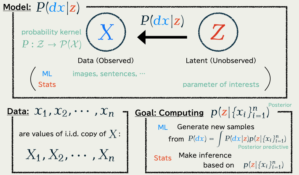
1.3 Markov Chain Monte Carlo

Property of Langevin Diffusion

d\textcolor{#2780e3}{X_t}=-\nabla\log p(\textcolor{#2780e3}{X_t}|\{x_i\}_{i=1}^n)\,dt+dB_t

converges to p(\textcolor{#E95420}{z}|\{x_i\}_{i=1}^n) as t\to\infty.

This approach is feasible because …

\text{score function}\quad\nabla\log p(\textcolor{#E95420}{z}|\{x_i\}_{i=1}^n)

is evaluatable.

1.4 Piecewise Deterministic Monte Carlo

• Better convergence
  (Andrieu and Livingstone, 2021)
• Better scalability
  (Bierkens et al., 2019)
• Numerical stability
  (Chevallier et al., 2025)

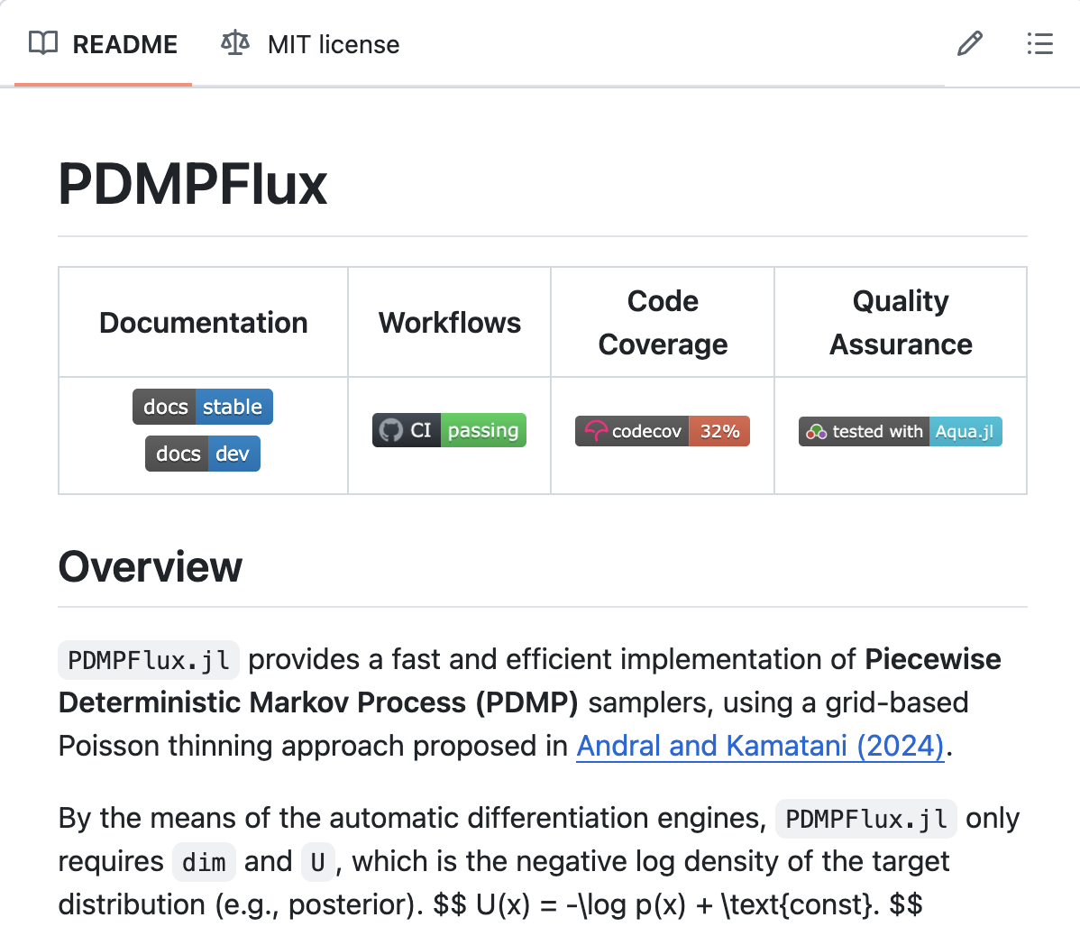
Available in our package PDMPFlux.jl

] add PDMPFlux

1.5 Variational Inference

\text{Posterior distribution:}\qquad p(\textcolor{#E95420}{z}|\boldsymbol{x})\propto p(\textcolor{#E95420}{z})\prod_{i=1}^n p(x_i|\textcolor{#E95420}{z}) is searched in a variational formulation via KL divergence: p(\textcolor{#E95420}{z}|\boldsymbol{x})=\argmin_{q\in\mathcal{P}(\textcolor{#E95420}{\mathcal{Z}})}\operatorname{KL}\bigg(q(\textcolor{#E95420}{z}),p(\textcolor{#E95420}{z}|\boldsymbol{x})\bigg).

Scalable Solution to VI

1. Constrain the problem on q\in\{q_{\textcolor{#E95420}{\phi}}\}_{\textcolor{#E95420}{\phi}\in\R^d},
2. Solve by (stochastic) optimization, using the gradient of \operatorname{KL}\bigg(q_{\textcolor{#E95420}{\phi}}(\textcolor{#E95420}{z}),p(\textcolor{#E95420}{z}|\boldsymbol{x})\bigg)=\operatorname{E}_{\textcolor{#E95420}{\phi}}[\log q_{\textcolor{#E95420}{\phi}}(\textcolor{#E95420}{Z})] -\operatorname{E}_{\textcolor{#E95420}{\phi}}[\log p(\textcolor{#E95420}{Z},\boldsymbol{x})]+\text{const.}

1.6 Variational Auto-Encoder (VAE)

In generative modeling, we also have to learn p\in\{p_{\textcolor{#2780e3}{\theta}}\}_{\textcolor{#2780e3}{\theta}\in\R^e}

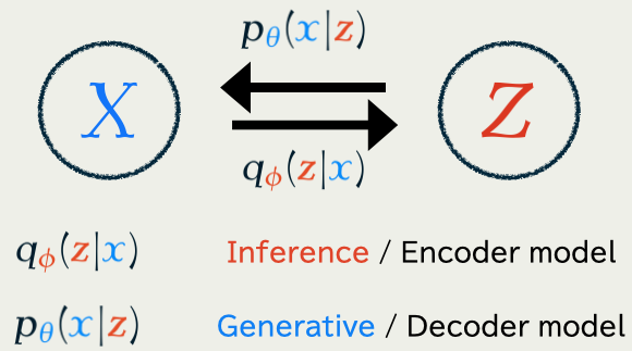
Jointly trained to minimize the KL divergence \operatorname{KL}\bigg(q_{\textcolor{#E95420}{\phi}}(\textcolor{#E95420}{z}|\textcolor{#2780e3}{x}),p_{\textcolor{#2780e3}{\theta}}(\textcolor{#E95420}{z}|\textcolor{#2780e3}{x})\bigg).

1.6 Variational Auto-Encoder (VAE)

(Kingma and Welling, 2014) found that a part of the KL divergence \begin{align*} &\operatorname{KL}\bigg(q_{\textcolor{#E95420}{\phi}}(\textcolor{#E95420}{z}|\textcolor{#2780e3}{x}),p_{\textcolor{#2780e3}{\theta}}(\textcolor{#E95420}{z}|\textcolor{#2780e3}{x})\bigg)\\ &\qquad=\operatorname{E}_{\textcolor{#E95420}{\phi},\textcolor{#2780e3}{x}}[\log q_{\textcolor{#E95420}{\phi}}(\textcolor{#E95420}{Z}|\textcolor{#2780e3}{x})] -\operatorname{E}_{\textcolor{#E95420}{\phi},\textcolor{#2780e3}{x}}[\log p_{\textcolor{#2780e3}{\theta}}(\textcolor{#E95420}{Z},\textcolor{#2780e3}{x})]+\log p_{\textcolor{#2780e3}{\theta}}(\textcolor{#2780e3}{x})\\ &\qquad=\underbrace{\operatorname{KL}\bigg(q_{\textcolor{#E95420}{\phi}}(\textcolor{#E95420}{z}|\textcolor{#2780e3}{x}),p_{\textcolor{#2780e3}{\theta}}(\textcolor{#E95420}{z})\bigg)-\operatorname{E}_{\textcolor{#E95420}{\phi},\textcolor{#2780e3}{x}}[\log p_{\textcolor{#2780e3}{\theta}}(\textcolor{#2780e3}{x}|\textcolor{#E95420}{Z})]}_{=:-\operatorname{ELBO}(\textcolor{#2780e3}{\theta},\textcolor{#E95420}{\phi})\text{ : we only optimize this part}}+\log p_{\textcolor{#2780e3}{\theta}}(\textcolor{#2780e3}{x}) \end{align*} still lends itself to stochastic optimization.

Once \textcolor{#2780e3}{\theta^*} is learned, we are able to sample from p_{\textcolor{#2780e3}{\theta^*}}(\textcolor{#2780e3}{x})=\int_{\textcolor{#E95420}{\mathcal{Z}}}p_{\textcolor{#2780e3}{\theta^*} }(\textcolor{#2780e3}{x}|\textcolor{#E95420}{z})p_{\textcolor{#2780e3}{\theta^*} }(\textcolor{#E95420}{z})\,d\textcolor{#E95420}{z}

Note that now q_{\textcolor{#E95420}{\phi}} depends on \textcolor{#2780e3}{x} as well.

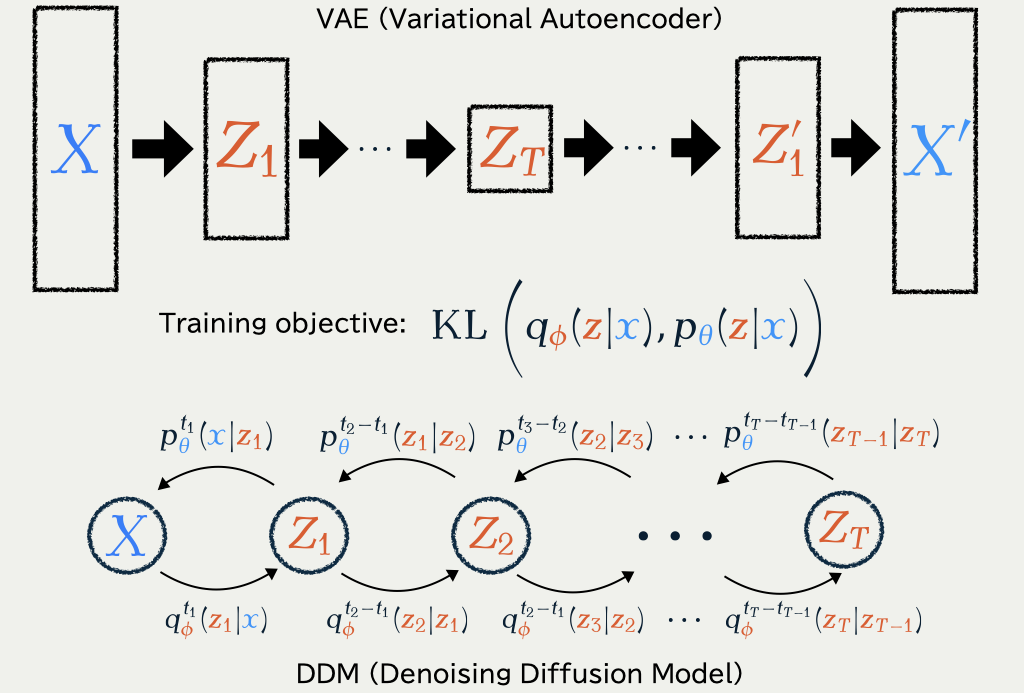
1.7 Denoising Diffusion Models (DDM)

Concentrating on learning p_{\textcolor{#2780e3}{\theta}}, we fix q_{\textcolor{#E95420}{\phi}}(\textcolor{#E95420}{z}|\textcolor{#2780e3}{x})=q(\textcolor{#E95420}{z}|\textcolor{#2780e3}{x})=q^{t_1}(\textcolor{#E95420}{z_1}|\textcolor{#2780e3}{x})\prod_{i=1}^T q^{t_{i+1}-t_i}(\textcolor{#E95420}{z_{i+1}}|\textcolor{#E95420}{z_{i}}), as a path measure of a Langevin diffusion on \textcolor{#E95420}{\mathcal{Z}}=(\R^d)^{T+1}.

A common choice is an OU process: q^t(z|x)=\operatorname{N}(z;x,t).

1.7 Denoising Diffusion Models (DDM)

As proposed in (Sohl-Dickstein et al., 2015), the KL will reduce to \begin{align*} \mathcal{L}(\textcolor{#2780e3}{\theta})&=\operatorname{KL}\bigg(q(\textcolor{#E95420}{z_{1:T}}|\textcolor{#2780e3}{x}),p_{\textcolor{#2780e3}{\theta}}(\textcolor{#E95420}{z_{1:T}}|\textcolor{#2780e3}{x})\bigg)\\ &=\operatorname{E}[\log q(\textcolor{#E95420}{Z_{1:T}}|\textcolor{#2780e3}{x})]-\operatorname{E}[\log p_{\textcolor{#2780e3}{\theta}}(\textcolor{#2780e3}{x},\textcolor{#E95420}{Z_{1:T}})]+\log p_{\textcolor{#2780e3}{\theta}}(\textcolor{#2780e3}{x})\\ &=:-\operatorname{ELBO}(\textcolor{#2780e3}{\theta})+\log p_{\textcolor{#2780e3}{\theta}}(\textcolor{#2780e3}{x}). \end{align*} By maximizing the \operatorname{ELBO}(\textcolor{#2780e3}{\theta}), we are still performing a form of (approximate) maximum likelihood inference since \operatorname{ELBO}(\textcolor{#2780e3}{\theta})\le\log p_{\textcolor{#2780e3}{\theta}}(\textcolor{#2780e3}{x}). Although approximate as inference, it proved to be very effective in generating high-quality images (Ho et al., 2020).

1.7 Denoising Diffusion Models (DDM)

It is because DDM learns how to denoise a noisy data. DDM …

× constrains the posterior to be \operatorname{N}(0,I_d),

○ the whole training objective is devoted to learn the generator p_{\textcolor{#2780e3}{\theta}}

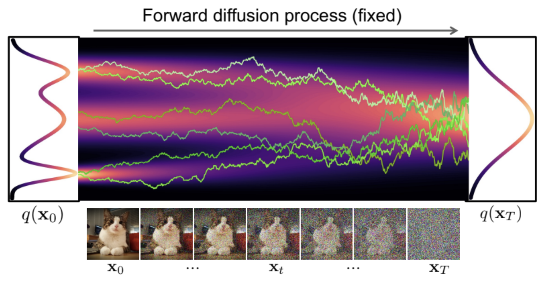
A very famous figure from (Kreis et al., 2022)

Summary

• Problem Setting: Generative Modeling ≒ Bayesian Modeling
• Two main approaches:
  • Sampling-based Methods: MCMC, PDMC, etc.
  • Optimization-based Methods: VI, VAE, DDM, etc.
• DDM succeeds by
  • Discarding modeling inference process q_{\textcolor{#E95420}{\phi}}
  • Concentrating on learning to generate from p_{\textcolor{#2780e3}{\theta}}

Development 1: More Concentration on Learning to Generate

Isn’t there a more suitable training objective?

Development 2: Overlooked Design Choice

Was “fixing q_{\textcolor{#E95420}{\phi}} to be a Langevin diffusion” really a good idea?

2 Developments in Continuous Diffusion Models

Historical Development

Data Space \textcolor{#2780e3}{\mathcal{X}}	Continuous	Discrete
Origin	(Ho et al., 2020)	(Austin et al., 2021)
Continuous-time	(Y. Song et al., 2021)	(Campbell et al., 2022)
Score-based	(Y. Song et al., 2021)	(Sun et al., 2023)
Flow-based	(Lipman et al., 2023)	(Gat et al., 2024)

2.1 Limit in T\to\infty leads to SDE formulation

2.2 Score-based DDM in SDE formulation

Theorem from (Anderson, 1982)

(\textcolor{#E95420}{Z}_t)_{t=0}^T and (\textcolor{#2780e3}{X}_{T-t})_{t=0}^T have the same path measure:

\text{\textcolor{#E95420}{Langevin diffusion}:}\qquad\qquad d\textcolor{#E95420}{Z}_t=b_t(\textcolor{#E95420}{Z}_t)\,dt+dB_t \text{\textcolor{#2780e3}{Denoising diffusion}:}\quad d\textcolor{#2780e3}{X}_t=\bigg(-b_{T-t}(\textcolor{#2780e3}{X}_t)+\underbrace{\nabla\log q^{T-t}(\textcolor{#2780e3}{X}_t)}_{\text{score function}}\bigg)\,dt+dB'_t

Learning (\textcolor{#2780e3}{X}_{t}) is equivalent to learning the score s_{\textcolor{#2780e3}{\theta}} by the loss \mathcal{L}(\textcolor{#2780e3}{\theta})=\int^T_0\operatorname{E}\bigg[\bigg|\nabla\log q^t(\textcolor{#E95420}{Z_t}|\textcolor{#2780e3}{x})-s_{\textcolor{#2780e3}{\theta}}(\textcolor{#E95420}{Z_t},t)\bigg|^2\bigg]\,dt.

This is proposed by (Y. Song et al., 2021). \mathcal{L}(\textcolor{#2780e3}{\theta}) is called the denoising score matching loss.

2.3 ODE Sampling of Score-based DDM

\text{ODE:}\qquad\frac{d\textcolor{#2780e3}{X}_t}{dt}=-b_t(\textcolor{#2780e3}{X_t})+\frac{1}{2}s_{\textcolor{#2780e3}{\theta}}^t(\textcolor{#2780e3}{X_t})=:v^t_\theta(\textcolor{#2780e3}{X_t}) \tag{1} has the same 1d marginal distributions as \text{\textcolor{#2780e3}{Denoising diffusion} SDE:}\quad d\textcolor{#2780e3}{X_t}=\bigg(-b_{t}(\textcolor{#2780e3}{X_t})+s_{\textcolor{#2780e3}{\theta}}^{t}(\textcolor{#2780e3}{X_t})\bigg)\,dt+dB_t.

2.4 New Loss Enables New Sampling

	SDE sampling	ODE sampling
Forward Path	(q^t(\textcolor{#E95420}{z}|\textcolor{#2780e3}{x}))_{t=0}^T	(q^t(\textcolor{#E95420}{z}|\textcolor{#2780e3}{x}))_{t=0}^T
Backward Path	(p^t_{\textcolor{#2780e3}{\theta}}(\textcolor{#2780e3}{x}|\textcolor{#E95420}{z}))_{t=0}^T	(?)
Speed	Slow	Fast
Quality	High	Low

Problem: “ODE Solver applied to SDE path” doesn’t make sense.

→ Explore other possibilities in the forward path

(Karras et al., 2022) uses Heun’s 2nd order correction method to discretize the ODE.

The ODE parametrization by (J. Song et al., 2021) is favorable from its stable curvature.

Discretizing the SDE by adding extra noise results in higher quality in imagenet dataset.

The SDE approach seems to be more robust to the estimation error in the score (Cao et al., 2023).

2.5 In Search of Better Forward Path

Discrete Time Markov Chain

Diffusion Process

Piecewise Deterministic

2.6 Flow-based DDM: A Flexible Framework

Instead of score \nabla\log q^t(\textcolor{#E95420}{z}), we learn the vector field u satisfying (\text{continuity equation})\quad\partial_tp^t+\operatorname{div}(p^tu^t)=0. We learn u by a NN (t,x)\mapsto v_{\textcolor{#2780e3}{\theta}}^t(x) with the loss \text{Flow Matching Loss:}\qquad\mathcal{L}_{\text{FM}}(\textcolor{#2780e3}{\theta})=\int_0^T\operatorname{E}\bigg[\bigg|v_{\textcolor{#2780e3}{\theta}}^t(X)-u^t(X)\bigg|^2\bigg]\,dt. To generate a new sample, we let X_0\sim p^0 flow along v_{\textcolor{#2780e3}{\theta^*}}^t.

Usually, FM is understood as a scalable alternative to train CNFs (Chen et al., 2018). Being an alternative to score matching by learning directly the RHS of (1), this approach is called flow matching, independently proposed by (X. Liu et al., 2023), (Albergo and Vanden-Eijnden, 2023), (Lipman et al., 2023).

2.7 From Path to Flow

Diffusion Path

p_{\textcolor{#2780e3}{\theta}}^t(-|\textcolor{#2780e3}{x})=\operatorname{N}\bigg(\alpha_{1-t}\textcolor{#2780e3}{x},(1-\alpha_{1-t}^2)I_d\bigg) corresponds to u_t(\textcolor{#E95420}{z}|\textcolor{#2780e3}{x})=\frac{\alpha_{1-t}}{1-\alpha_{1-t}^2}(\alpha_{1-t}\textcolor{#E95420}{z}-\textcolor{#2780e3}{x})

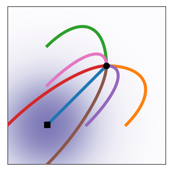
Optimal Transport Path

p_{\textcolor{#2780e3}{\theta}}^t(-|\textcolor{#2780e3}{x})=\operatorname{N}\bigg(t\textcolor{#2780e3}{x},(1-t)I_d\bigg) corresponds to u_t(\textcolor{#E95420}{z}|\textcolor{#2780e3}{x})=\frac{\textcolor{#2780e3}{x}-\textcolor{#E95420}{z}}{1-t}

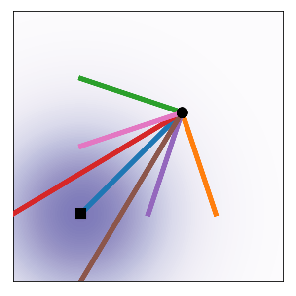
OT paths result in straight trajectries with constant speed, which is more suitable for stable generation.

Figures are from (Lipman et al., 2023).

Summary: Towards Straighter Paths

• SDE formulation enables faster ODE sampling
• ODE sampling is possible to other choices of q_{\textcolor{#E95420}{\phi}}
  \because\quad Only 1d marginals matter (= Flow-based Modeling)
  • Langevin path ← the Diffusion Model
  • Optimal Transport path
  • more in discrete settings!

Langevin Path

ODE Path w.r.t. Langevin Forward

OT Path

3 Discrete Diffusion Models

Block Diffusion proposed in (Arriola et al., 2025)

3.1 Masking Processes

with some rate R_t(\texttt{mask}|x)>0 of masking x\ne\texttt{mask}.

The reverse process is characterized by the rate \textstyle\hat{R}_t(x|y)=R_t(y|x)\underbrace{\frac{q^t(x)}{q^t(y)}.}_{\text{learn this part using NN}}

Comparison of forward designs (Liang et al., 2025)

Forward process	Uniform	Masking
Number of steps needed in backward process	\tilde{O}(d^2/\epsilon)	\tilde{O}(d/\epsilon)

This continuous-time approach starts with (Campbell et al., 2022), followed by (Sun et al., 2023) and culminates in (Lou et al., 2024).

3.2 Discrete Flow Matching

Targets a forward process \{q_t\}_{t=0}^T\subset\mathcal{P}(\textcolor{#E95420}{\mathcal{Z}}\sqcup\{\texttt{mask}\}) that satisfies \text{linear interpolation:}\qquad q_t(-|\textcolor{#2780e3}{x})=(1-\alpha_t)\delta_{\textcolor{#2780e3}{x}}(-)+\alpha_t\delta_{\texttt{mask}}(-), A backward sampling process is given by \text{rate function:}\qquad R_t(\textcolor{#2780e3}{x}|\mathtt{mask})=\frac{\dot{\alpha}_t}{1-\alpha_t}\underbrace{p^t(\textcolor{#2780e3}{x}|\mathtt{mask}).}_{\text{learn this part using NN}} The predictor p^t(\textcolor{#2780e3}{x}|\mathtt{mask}) is learned by the loss \mathcal{L}(\textcolor{#2780e3}{\theta})=\int^T_0\frac{\dot{\alpha}_t}{1-\alpha_t}\operatorname{E}\bigg[\operatorname{KL}\bigg(p^{\text{\textcolor{#2780e3}{data}}},p^t_{\textcolor{#2780e3}{\theta}}(\textcolor{#2780e3}{X_t}|\texttt{mask})\bigg)\bigg]\,dt.

Theory lacks in this setting.

This approach culminates in (Shi et al., 2024), (S. Liu et al., 2025).

References

Albergo, M. S., and Vanden-Eijnden, E. (2023). Building Normalizing Flows with Stochastic Interpolants. In The eleventh international conference on learning representations.

Anderson, B. D. O. (1982). Reverse-time diffusion equation models. Stochastic Processes and Their Applications, 12(3), 313–326.

Andrieu, C., and Livingstone, S. (2021). Peskun–Tierney ordering for Markovian Monte Carlo: Beyond the reversible scenario. The Annals of Statistics, 49(4), 1958–1981.

Arriola, M., Sahoo, S. S., Gokaslan, A., Yang, Z., Qi, Z., Han, J., … Kuleshov, V. (2025). Block diffusion: Interpolating between autoregressive and diffusion language models. In The thirteenth international conference on learning representations.

Austin, J., Johnson, D. D., Ho, J., Tarlow, D., and Berg, R. van den. (2021). Structured Denoising Diffusion Models in Discrete State-Spaces. In M. Ranzato, A. Beygelzimer, Y. Dauphin, P. S. Liang, and J. W. Vaughan, editors, Advances in neural information processing systems,Vol. 34, pages 17981–17993. Curran Associates, Inc.

Bierkens, J., Fearnhead, P., and Roberts, G. (2019). The Zig-Zag Process and Super-Efficient Sampling for Bayesian Analysis of Big Data. The Annals of Statistics, 47(3), 1288–1320.

Campbell, A., Benton, J., De Bortoli, V., Rainforth, T., Deligiannidis, G., and Doucet, A. (2022). A continuous time framework for discrete denoising models. In S. Koyejo, S. Mohamed, A. Agarwal, D. Belgrave, K. Cho, and A. Oh, editors, Advances in neural information processing systems,Vol. 35, pages 28266–28279. Curran Associates, Inc.

Cao, Y., Chen, J., Luo, Y., and ZHOU, X. (2023). Exploring the optimal choice for generative processes in diffusion models: Ordinary vs stochastic differential equations. In A. Oh, T. Naumann, A. Globerson, K. Saenko, M. Hardt, and S. Levine, editors, Advances in neural information processing systems,Vol. 36, pages 33420–33468. Curran Associates, Inc.

Chen, R. T. Q., Rubanova, Y., Bettencourt, J., and Duvenaud, D. K. (2018). Neural ordinary differential equations. In S. Bengio, H. Wallach, H. Larochelle, K. Grauman, N. Cesa-Bianchi, and R. Garnett, editors, Advances in neural information processing systems,Vol. 31. Curran Associates, Inc.

Chevallier, A., Power, S., and Sutton, M. (2025). Towards practical PDMP sampling: Metropolis adjustments, locally adaptive step-sizes, and NUTS-based time lengths.

Gat, I., Remez, T., Shaul, N., Kreuk, F., Chen, R. T. Q., Synnaeve, G., … Lipman, Y. (2024). Discrete flow matching. In A. Globerson, L. Mackey, D. Belgrave, A. Fan, U. Paquet, J. Tomczak, and C. Zhang, editors, Advances in neural information processing systems,Vol. 37, pages 133345–133385. Curran Associates, Inc.

Ho, J., Jain, A., and Abbeel, P. (2020). Denoising Diffusion Probabilistic Models. In Advances in neural information processing systems,Vol. 33.

Karras, T., Aittala, M., Aila, T., and Laine, S. (2022). Elucidating the design space of diffusion-based generative models. In A. H. Oh, A. Agarwal, D. Belgrave, and K. Cho, editors, Advances in neural information processing systems.

Kingma, D. P., and Welling, M. (2014). Auto-encoding variational bayes. In International conference on learning representations,Vol. 2.

Kreis, K., Gao, R., and Vahdat, A. (2022). Denoising diffusion-based generative modeling: Foundations and applications.

Liang, Y., Huang, R., Lai, L., Shroff, N., and Liang, Y. (2025). Absorb and converge: Provable convergence guarantee for absorbing discrete diffusion models.

Lipman, Y., Chen, R. T. Q., Ben-Hamu, H., Nickel, M., and Le, M. (2023). Flow matching for generative modeling. In The eleventh international conference on learning representations.

Liu, S., Nam, J., Campbell, A., Stark, H., Xu, Y., Jaakkola, T., and Gomez-Bombarelli, R. (2025). Think while you generate: Discrete diffusion with planned denoising. In The thirteenth international conference on learning representations.

Liu, X., Gong, C., and liu, qiang. (2023). Flow straight and fast: Learning to generate and transfer data with rectified flow. In The eleventh international conference on learning representations.

Lou, A., Meng, C., and Ermon, S. (2024). Discrete diffusion modeling by estimating the ratios of the data distribution. In R. Salakhutdinov, Z. Kolter, K. Heller, A. Weller, N. Oliver, J. Scarlett, and F. Berkenkamp, editors, Proceedings of the 41st international conference on machine learning,Vol. 235, pages 32819–32848. PMLR.

Neklyudov, K., Brekelmans, R., Severo, D., and Makhzani, A. (2023). Action matching: Learning stochastic dynamics from samples. In A. Krause, E. Brunskill, K. Cho, B. Engelhardt, S. Sabato, and J. Scarlett, editors, Proceedings of the 40th international conference on machine learning,Vol. 202, pages 25858–25889. PMLR.

Ryu, S. (2024). Minimal implementation of a D3PM (structured denoising diffusion models in discrete state-spaces), in pytorch.

Shi, J., Han, K., Wang, Z., Doucet, A., and Titsias, M. (2024). Simplified and generalized masked diffusion for discrete data. In A. Globerson, L. Mackey, D. Belgrave, A. Fan, U. Paquet, J. Tomczak, and C. Zhang, editors, Advances in neural information processing systems,Vol. 37, pages 103131–103167. Curran Associates, Inc.

Sohl-Dickstein, J., Weiss, E., Maheswaranathan, N., and Ganguli, S. (2015). Deep Unsupervised Learning using Nonequilibrium Thermodynamics. In F. Bach and D. Blei, editors, Proceedings of the 32nd international conference on machine learning,Vol. 37, pages 2256–2265. Lille, France: PMLR.

Song, J., Meng, C., and Ermon, S. (2021). Denoising diffusion implicit models. In International conference on learning representations.

Song, Y., Sohl-Dickstein, J., Kingma, D. P., Kumar, A., Ermon, S., and Poole, B. (2021). Score-Based Generative Modeling through Stochastic Differential Equations. In International conference on learning representations.

Sun, H., Yu, L., Dai, B., Schuurmans, D., and Dai, H. (2023). Score-based continuous-time discrete diffusion models. In The eleventh international conference on learning representations.

Appendix

Algorithmic Stability

The Score of DDM (Y. Song et al., 2021)

The Vector Field of FM (Lipman et al., 2023)

One hidden theme was algorithmic stability, which plays a crucial role in the successful methods.

Other Training Objectives

Instead of the vector field u, we can learn its potential v_\theta^t=\nabla s_\theta^t. through the Action Matching loss (Neklyudov et al., 2023) \mathcal{L}_{\text{AM}}(\theta)=\operatorname{E}[s^0_\theta(X_0)-s^1_\theta(X_1)]+\int^1_0\operatorname{E}\bigg[\frac{1}{2}|\nabla s^t_\theta(X)|^2+\partial_ts^t_\theta(X)\bigg]\,dt