Implementation Details of PDMPFlux.jl

1 Introduction

In this introduction, we quickly give an overview of how the PDMPFlux.jl package works, through a standard example.

Take the Sticky Zig-Zag Sampler (Bierkens et al., 2023) as an example.

1. sampler = StickyZigZag(dim, ∇U)

   This instantiates the sampler, an object of an AbstractPDMP subtype.

2. output = sample_skeleton(sampler, N_sk, xinit, vinit)

   This takes a sampler object, and returns a PDMPHistory object, by transforming the PDMPState object while pushing its snapshots into the PDMPHistory object.

2 Directory Structure of PDMPFlux.jl/src

2.1 Composites.jl

composites / constructs such as BoundBox, PDMPState, PDMPHistory are defined.

• BoundBox is basically a grid, together with the values on it, tailored to perform Poisson thinning. 3 constructors are defined in UpperBound.jl Section 2.4.

  • boundbox.grid is the grid points. Let the dimension be n_grid, which is a field of any AbstractPDMP subtype.
  • The grid is equi-spaced, with the step size step_size.
  • boundbox.box_max has n_grid - 1 elements \[ \textcolor{purple}{\mathtt{box\_max[i]}} = \max_{t \in [\textcolor{purple}{\mathtt{grid[i]}}, \textcolor{purple}{\mathtt{grid[i+1]}}]} \lambda(t),\qquad i\in[\textcolor{purple}{\mathtt{n\_grid-1}}]. \]
  • boundbox.cum_sum has n_grid elements, and \[ \textcolor{purple}{\mathtt{cum\_sum[i]}} = \sum_{j=1}^{i-1} \textcolor{purple}{\mathtt{box\_max[j]}}\times\textcolor{purple}{\mathtt{step\_size}},\qquad i\in[\textcolor{purple}{\mathtt{n\_grid}}]. \] Note that it is not the cumulative sum of box_max, but the cumulative sum of the piecewise constant (upper bound) function represented by box_max’s: \[ \textcolor{purple}{\mathtt{cum\_sum[i]}} = \int^i_0\sum_{j=1}^{\textcolor{purple}{\mathtt{n\_grid}-1}}1_{[\textcolor{purple}{\mathtt{grid[j]}}, \textcolor{purple}{\mathtt{grid[j+1]}})}(t)\cdot\textcolor{purple}{\mathtt{box\_max[j]}}\,dt,\qquad i\in[\textcolor{purple}{\mathtt{n\_grid}}]. \]

• PDMPState is used to keep the position of the sampler, together with caracteristics and diagnostic information. The whole SamplingLoop.jl Section 2.3 is implemented as a collection of functions that modify the PDMPState object in place. In addition to the \((x,v,t)\) tuple, the fields include

  • methods specific to the sampler.
    • state.rate and state.rate_vect are the rate function and its vectorized version. These slots are determined after checking the field pdmp.signed_bound in init_state() in AbstractPDMP.jl Section 3.2.
    • state.upper_bound_func() takes \((x,v,t)\) and returns the BoundBox object. Basically, state.upper_bound_func() is the only field that differs among samplers.
    • state.velocity_jump() takes \((x,v,t)\) and returns the velocity vector after the PDMP’s jump.
    • state.flow() takes \((x_0,v_0,t)\) and returns \((x_t,v_t)\), which indicates the PDMP’s position after the time \(t\) from \((x_0,v_0)\).
  • fields to facilitate the sampling loop.
    • boolean flags to indicate whether Poisson thinning proposal is accepted or not, which is used within ac_step_with_proxy() in the SamplingLoop.jl Section 2.3.
    • proposed jump time tp and time already spent ts. They are using in SamplingLoop.jl Section 2.3 to conduct poisson thinning, where tp is the proposed jump time, and is added to ts when rejected.
    • horizon is passed to upper-bounding functions to create a BoundBox object.
  • statistics to diagnose the sampler dynamic.

2.2 sample.jl

sample.jl contains functions, called by users, to start MCMC sampling. The ProgressBar package is used to be friendly to users.

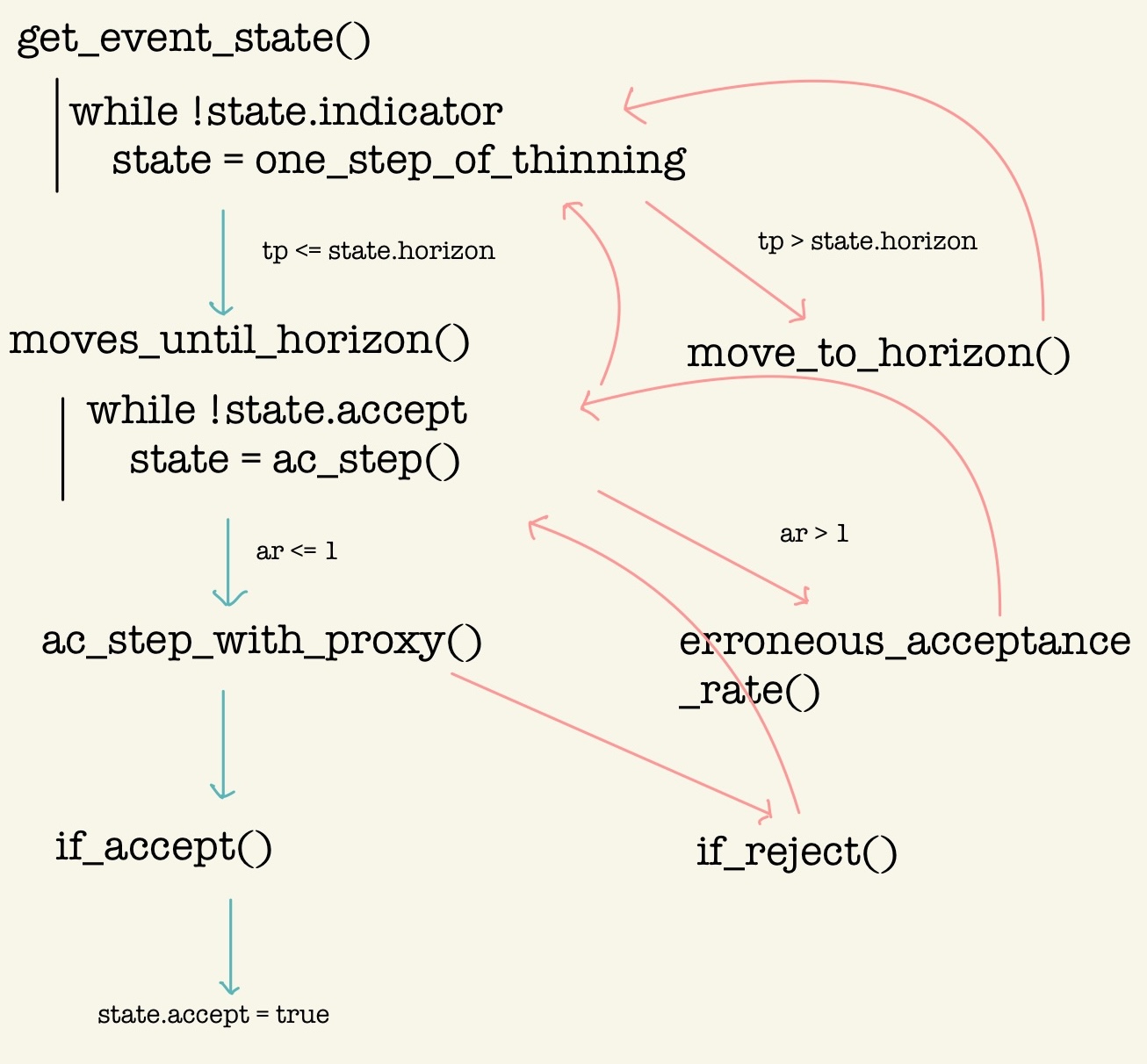
sample.jl contains 2 functions, and sample() that calls them in sequel.

• sample_skeleton() -> PDMPHistory initializes the progress bar and PDMPState & PDMPHistory objects, using init_state() and PDMPHistory() constructor respectively. Then call get_event_state() in SamplingLoop.jl Section 2.3 for iter::Int times.
• sample_from_skeleton() -> Matrix{Float64} is a function that generates samples, which might subsequently be called by the plotting functions in plot.jl.

2.3 SamplingLoop.jl

This module contains 10 functions. Some of them are summarized in the following figure:

The main loop for sampling is implemented here.

• get_event_state() -> PDMPState is the entering point from sample.jl.

  • There is only one thing in get_event_state(), i.e., callling one_step_of_thinning() until state.accept becomes true.

  • get_event_state() returns a PDMPState object with the field \((x,v,t)\) indicating where an accepted event happens, which is pushed to PDMPHistory back in sample_skeleton() in sample.jl Section 2.2.

• one_step_of_thinning() returns where simulation has completed up to, with state.accept = false if any proposal isnot accepted yet.

  • Firstly, it proposes the next jump event, by simulating exp_rv and calling next_event(upper_bound, exp_rv) -> (tp, lambda_bar).

    • upper_bound is the BoundBox object, which is calculated by state.upper_bound_func() and the current state (x,v,t).
    • tp is the proposed jump time.
    • lambda_bar is a upper bound, with error, for the rate function \(\lambda\).

  • Secondly, it checks whether tp <= state.horizon.

    • If not, it calls move_to_horizon() and continues the loop one_step_of_thinning() inside get_event_state().
    • If yes, it proceeds to moves_until_horizon(), where another loop, calling ac_step(), is performed until one of the following 2 happens
      • when state.accept becomes true, it gets out of the both loops.
      • when tp > state.horizon, it calls move_to_horizon2() to get out of ac_step() loop, and continues the loop one_step_of_thinning() inside get_event_state().

• ac_step(), standing for acceptance-rejection step, is the core of Poisson thinning.

  • calculating the acceptance rate ar, which might exceed \(1.0\).

    In that case, erroneous_acceptance_rate() is called to shrink the horizon by half, and then continues the ac_step() loop in moves_until_horizon() function. Shrinking horizon leads to a finer grid, since n_grid is fixed.

  • Otherwise, it performs the Poisson thinning using the proxy rate lambda_bar, in ac_step_with_proxy() call.

    • Within ac_step_with_proxy(), either if_accept() or if_reject() is called depending on the result of Poisson thinning, followed by move_to_horizon2() if accepted. Whether accepted or not is informed by state.accept flag, which will lead you out of all the loops.
    • In if_accept(), the flags are updated as state.accept = true & state.accept = true, getting out of both ac_step() loop and one_step_of_thinning() loop, with the correct \((x,v,t)\) stored in appropriate state’s fields, which is pushed to PDMPHistory back in sample_skeleton() in sample.jl Section 2.2.
    • if_reject() being called, we are still in the ac_step() loop in moves_until_horizon(), until acceptance or tp > state.horizon.

2.4 UpperBound.jl

This module contains next_event() function and 3 constructors for BoundBox object, with the name of upper_bound_**().

3 constructors for BoundBox object

upper_bound_**(func::Function, start::Float64, horizon::Float64) -> BoundBox

• upper_bound_constant() computes the constant upper bound for the function func over the interval [start, horizon].

  Technically, it returns the BoundBox object, with just 2 grid points, start and horizon. The maximum value is searched by the Brent’s algorithm via Optim.jl package.

• upper_bound_grid() computes a piecewise constant upper bound, using the n_grid grid points.

  The box_max[i] field is the maximum value of the three points in the interval [grid[i], grid[i+1]], which are the values on the two edges func(grid[i]), func(grid[i+1]), and the intersection point of the two tangents on the two edges of the interval.

• upper_bound_grid_vect() is a LinearAlgebra implementation of upper_bound_grid().

next_event(boundbox, exp_rv) takes boundbox to propose a next event time

index = searchsortedfirst(boundbox.cum_sum, exp_rv)

is performed to find the index that satisfies

\[ \textcolor{purple}{\mathtt{exp\_rv}} \in \left[\textcolor{purple}{\mathtt{cum\_sum[index-1]}}, \textcolor{purple}{\mathtt{cum\_sum[index]}}\right). \]

Finally, t_prop that satisfies

\[ \int^\textcolor{purple}{\mathtt{t\_prop}}_0 \overline{\lambda}(t)\,dt = \textcolor{purple}{\mathtt{exp\_rv}}, \] where \(\overline{\lambda}(t)\) is the piecewise constant upper-bounding function defined by \[ \overline{\lambda}(t) = \sum_{j=1}^{\textcolor{purple}{\mathtt{n\_grid}-1}}1_{[\textcolor{purple}{\mathtt{grid[j]}}, \textcolor{purple}{\mathtt{grid[j+1]}})}(t)\cdot\textcolor{purple}{\mathtt{box\_max[j]}}. \]

next_event() returns the jump time t_prop and the corresponding upper bound value upper_bound, i.e., \[ \textcolor{purple}{\mathtt{upper\_bound}} = \overline{\lambda}(\textcolor{purple}{\mathtt{t\_prop}}) = \textcolor{purple}{\mathtt{box\_max[index-1]}}. \]

2.5 diagnostic.jl

function anim_traj(
    history::PDMPHistory, 
    N_max::Int; 
    N_start::Int=1, 
    plot_start::Int=1, 
    filename::Union{String, Nothing}=nothing, 
    plot_type="2D", 
    color="#78C2AD", 
    background="#FFF", 
    coordinate_numbers=[1,2,3], 
    dt::Float64=0.1, 
    verbose::Bool=true, 
    fps::Int=60, 
    frame_upper_limit::Int=10000, 
    linewidth=2, 
    dynamic_range::Bool=false
)

arguments of anim_traj()

• history takes the output of sample_skeleton().
• N_start, N_max are the indeces of history to be plotted. Namely, from N_start th event, including reflection, refreshing, and thawing events, to N_max th event.
• plot_start is the starting index of the animation. The points of history.x[1:plot_start] will be already there in the first frame of the animation.
• frame_upper_limit is the maximum number of frames to be plotted.
• fps is the frame rate of the animation.
• dynamic_range is a boolean flag to determine whether to use the dynamic range for the animation.

2.6 plot.jl

This file contains functions to plot the samples generated by sample.jl.

3 Implementation of the Samplers

3.1 Introduction

All samplers are defined as subtypes of AbstractPDMP in Samplers/AbstractPDMP.jl Section 3.2.

Different samplers have four different fields in PDMPState object, which are upper_bound_func, rate, rate_vect, and velocity_jump, as we learned in Section 2.1.

The four special fields are initialized in the constructor defined in the respective Samplers/<Name>.jl module.

3.2 Samplers/AbstractPDMP.jl

This module contains one line

abstract type AbstractPDMP end

and one function, whose signature is

init_state(pdmp::AbstractPDMP, xinit::Array{Float64}, vinit::Array{Float64}, seed::Int) -> PDMPState

This init_state() is basically a constructor for PDMPState, called in sample_skeleton() Section 2.2.

It is defined in AbstractPDMP.jl because the composite PDMPState must have different field values depending on the type of the argument pdmp.

init_state() mainly does two things

1. Check the field pdmp.signed_bound and modify the 3 fields rate, rate_vect, refresh_rate accordingly, which were already initialized in the respective constructor of pdmp.
2. Check the field pdmp.grid_size & pdmp.vectorized_bound and initialize the field upper_bound_func as one of the functions in the UpperBound.jl Section 2.4 module accordingly.

The remaining special fields, velocity_jump and flow are defined, together with initialization of rate and rate_vect, in the sampler specific modules, to which we will turnin the following sections.

3.3 Samplers/ZigZagSamplers.jl

In this module, the declaration

mutable struct ZigZag <: AbstractPDMP

is followed by the 2 constructors, ZigZag() and ZigZagAD(), whose signatures are

function ZigZag(dim::Int, ∇U::Function; refresh_rate::Float64=0.0, grid_size::Int=10, tmax::Union{Float64, Int}=2.0, 
                    vectorized_bound::Bool=true, signed_bound::Bool=true, adaptive::Bool=true)
function ZigZagAD(dim::Int, U::Function; refresh_rate::Float64=0.0, grid_size::Int=10, tmax::Union{Float64, Int}=2.0, 
                    vectorized_bound::Bool=true, signed_bound::Bool=true, adaptive::Bool=true, AD_backend::String="Zygote")

Notice the difference in ∇U and U in the arguments.

In ZigZag() and ZigZagAD(), two fields are initialized

1. flow is defined as

\[ \textcolor{purple}{\mathtt{flow}}\,(x_0,v_0,t) =(x_0+v_0t, v_0) \]

2. rate_vect is defined component-wisely as

   \[ \textcolor{purple}{\mathtt{rate\_vect[i]}}(x_0,v_0,t) = \max(0, \nabla U_i(x_0+v_0t)v_0), \] where \(\nabla U=(\nabla U_1,\dots,\nabla U_d)^\top\) is the gradient \(\nabla U:\mathbb{R}^d\to\mathbb{R}^d\).

   rate is the sum of rate_vect, i.e.,

   \[ \textcolor{purple}{\mathtt{rate}}(x_0,v_0,t) = \sum_{i=1}^d \textcolor{purple}{\mathtt{rate\_vect[i]}}(x_0,v_0,t). \]

   signed_rate_vect is a version of rate_vect without taking the max with \(0\).

Two flags signed_bound and vectorized_bound are true in default, in which case signed_rate_vect is used.

This is called the signed strategy, detailed in (Section 4.4.2 Andral and Kamatani, 2024).

The vectorized_bound is also special to the Zig-Zag samplers.

3.4 Samplers/BouncyParticleSamplers.jl

Similar to the Zig-Zag samplers, mutable struct BPS and 2 constructors BPS() and BPSAD() are defined.

Difference is that, in BPS, vectorization is not used, therefore vectorized_bound=false no matter what the user specifies.

Note that typically Bouncy Particle Samplers need nonzero refresh rate, therefore refresh_rate=0.0 would result in erronous samples.

3.5 Samplers/ForwardEventChainMonteCarlo.jl

Forward ECMC (Event Chain Monte Carlo) is a generalizatione of the Bouncy Particle Sampler, being free from the need of refreshing, substituting it with a ‘informed’ velocity jump.

Regarding the implementation, however, note there is an error in the pseudo-code of (Michel et al., 2020)’s paper, and in the implementation of the pdmp_jax package.

To sum it up, the velocity jump is implemented separately on \(\mathbb{R}\nabla U\) and \((\mathbb{R}\nabla U)^\perp\). To the former, the velocity is newly sampled from the invariant distribution directly, while to the latter, occasionally (tuned by mix_p) only two dimensions of them are changed. (If ran_p=false, they are swaped.)

As a result, the sampler loses ergodicity and confined to a certain subspace when, for example, \(U\) is completely isotropic and the initial velocity is proportional to its contours.

3.6 Samplers/StickyZigZagSamplers.jl

This module implements the Sticky Zig-Zag sampler, for variable selection with the spike-and-slab prior.

The sampler takes additional argument κ, which has to be positive Float64 or Inf, determining the ‘stickyness’ of the sampler.

3.7 StickySamplingLoops.jl

StickyPDMP samplers have their own sampling loop, implemented in StickySamplingLoops.jl using multiple dispatch.

• In one step of one_step_of_thinning_or_sticking_or_thawing(), it is first checked whether the sampler crosses any axes by \(\min(\textcolor{purple}{\mathtt{tp}}, \textcolor{purple}{\mathtt{tt}}, \textcolor{purple}{\mathtt{horizon}})0\).
  • If it does cross, move_to_axes_and_stick() is called.
  • Else, \(\min(\textcolor{purple}{\mathtt{tp}}, \textcolor{purple}{\mathtt{tt}}) > \textcolor{purple}{\mathtt{horizon}}\) is checked.
    • If it is true, move_to_horizon() is called.
  • Else, moves_until_horizon_or_axes() is called.

References

Andral, C., and Kamatani, K. (2024). Automated techniques for efficient sampling of piecewise-deterministic markov processes.

Bierkens, J., Grazzi, S., Meulen, F. van der, and Schauer, M. (2023). Sticky PDMP Samplers for Sparse and Local Inference Problems. Statistics and Computing, 33(1), 8.

Michel, M., Durmus, A., and Sénécal, S. (2020). Forward event-chain monte carlo: Fast sampling by randomness control in irreversible markov chains. Journal of Computational and Graphical Statistics, 29(4), 689–702.