PDMPFlux.jl パッケージ

1 速習 PDMP

1.1 はじめに

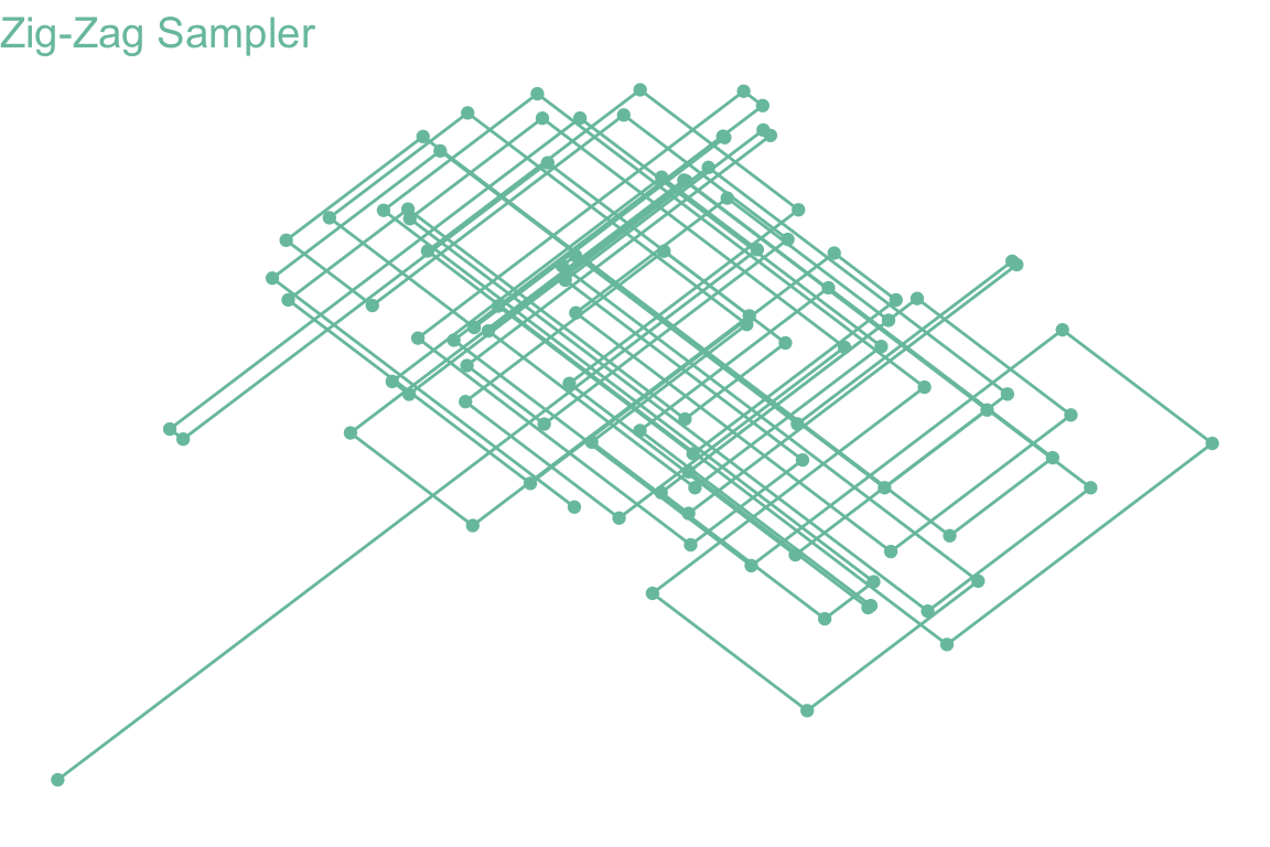
PDMP (Piecewise Deterministic Markov Process) または 連続時間 MCMC とは，名前の通り MCMC のサンプリングを連続時間で行うアルゴリズムである：

Zig-Zag サンプラーが２次元の正規分布からサンプリングを実行している様子

TipPDMP サンプラーの特徴

• 方向転換をするオレンジ色の点を一定の法則（Poisson 点過程）に従って定めることで，軌跡全体が目標の分布に従う．

• 目標の関数を緑色の軌跡上で線積分をすれば期待値が得られる．一定のステップサイズで切り出してサンプルとし，従来の MCMC output と同様に使っても良い．

• 非可逆 なダイナミクスをもち，HMC や MALA などの可逆なサンプラーよりも高次元分布や多様性に強いと期待されている．

詳しくは次の記事も参照：

A Blog Entry on Bayesian Computation by an Applied Mathematician

$$

$$

1.2 使い方

using PDMPFlux

Tip自動微分を使う場合（推奨）

1. まずポテンシャル＝負の対数尤度を（定数倍の違いを除いて）自分で定義する：

   function U_Gauss(x::Vector)
       return sum(x.^2) / 2
   end

   標準正規分布 \(\mathrm{N}_d(0,I_d)\) だと，対数尤度は \[ \log\phi(x) = - \frac{1}{2}\sum_{i=1}^d x_i^2 - \frac{d}{2}\log(2\pi) \] 第二項は定数であるから無視して良い．\(U(x) = -\log\phi(x)\) とすべき点に注意（先頭のマイナス符号は落とす）．

2. 次のようにしてサンプラーをインスタンス化する：

   dim = 10
   sampler = ZigZagAD(dim, U_Gauss)

3. ハイパーパラメータを与えてサンプリングを実行する．

   N_sk, N, xinit, vinit = 1_000_000, 1_000_000, zeros(dim), ones(dim)
   samples = sample(sampler, N_sk, N, xinit, vinit, seed=2024)

4. 結果の可視化を行う．

   jointplot(samples)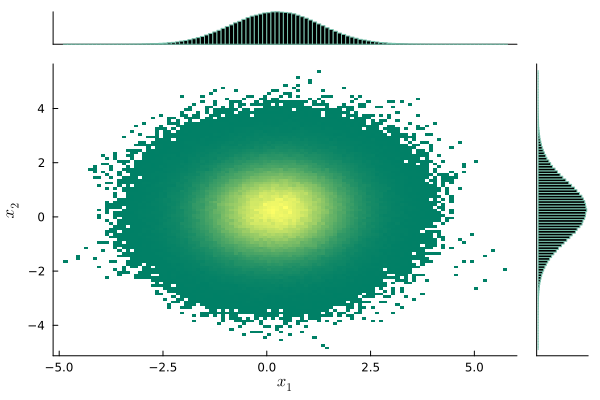

Tip自動微分を使わず，ポテンシャルの勾配を手動で与える場合

sampler = ZigZag(dim, grad_U, grid_size=grid_size)  # initialize your Zig-Zag sampler
output = sample_skeleton(sampler, N_sk, xinit, vinit, verbose = true)  # simulate skeleton points
samples = sample_from_skeleton(sampler, N, output)  # get samples from the skeleton points

とできる．

output::PDMPHistory にはサンプラーの挙動を確認するための多くのメソッドが定義されている：

plot_traj(output, 10000)
diagnostic(output)

2 pdmp_jax パッケージ

本節では PDMP のシミュレーションに自動微分を応用した (Andral and Kamatani, 2024) のアルゴリズムを紹介する．

2.1 デモ

(Neal, 2003) が slice sampling のデモ用に定義した 漏斗分布 を考える： \[ p(y,x)=\phi(y;0,3)\prod_{i=1}^9\phi(x_i;0,e^{y/2}),\qquad y\in\mathbb{R},x\in\mathbb{R}^9. \]

import jax
from jax.scipy.stats import multivariate_normal
from jax.scipy.stats import norm

import jax.numpy as jnp

def funnel(d=10, sig=3, clip_y=11):
  """Funnel distribution for testing. Returns energy and sample functions."""

  def unbatched(x):
    y = x[0]
    log_density_y = - y**2 / 6

    variance_other = jnp.exp(y/2)

    log_density_other = - jnp.sum(x[1:]**2) / (2 * variance_other)

    return - log_density_y - log_density_other

  def sample_data(n_samples):
    # sample from Nd funnel distribution
    y = (sig * jnp.array(np.random.randn(n_samples, 1))).clip(-clip_y, clip_y)
    x = jnp.array(np.random.randn(n_samples, d - 1)) * jnp.exp(-y / 2)
    return jnp.concatenate((y, x), axis=1)

  return unbatched, sample_data

import pdmp_jax as pdmp
dim = 10
U, _ = funnel(d=dim)
grad_U = jax.grad(U)
seed = 8
xinit = jnp.ones((dim,)) # initial position
vinit = jnp.ones((dim,))  # initial velocity
grid_size = 0
N_sk = 100000 # number of skeleton points
N = 100000 # number of samples
sampler = pdmp.ZigZag(dim, grad_U, grid_size)
# sample the skeleton of the process
out = sampler.sample_skeleton(N_sk, xinit, vinit, seed, verbose = True)  # takes only 3 seconds on my M1 Mac
# sample from the skeleton
sample = sampler.sample_from_skeleton(N,out)

import seaborn as sns
sns.jointplot(x = sample[:,0],y = sample[:,1])
plt.show()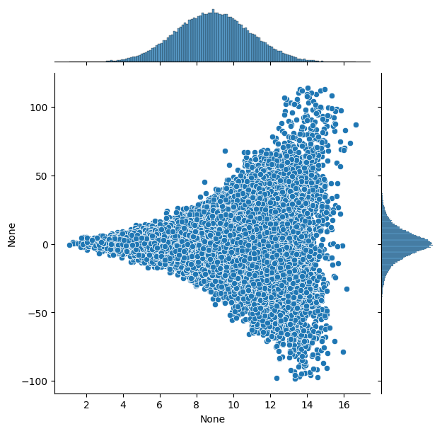

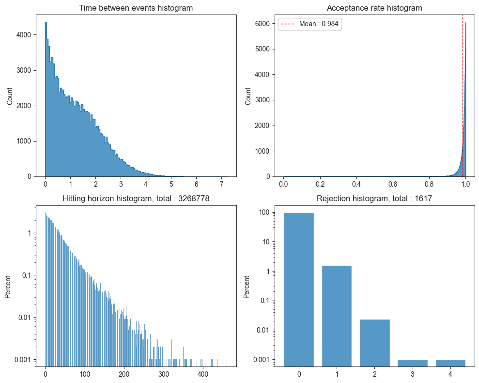
number of error bound : 46817

2.2 サンプリングループの構造

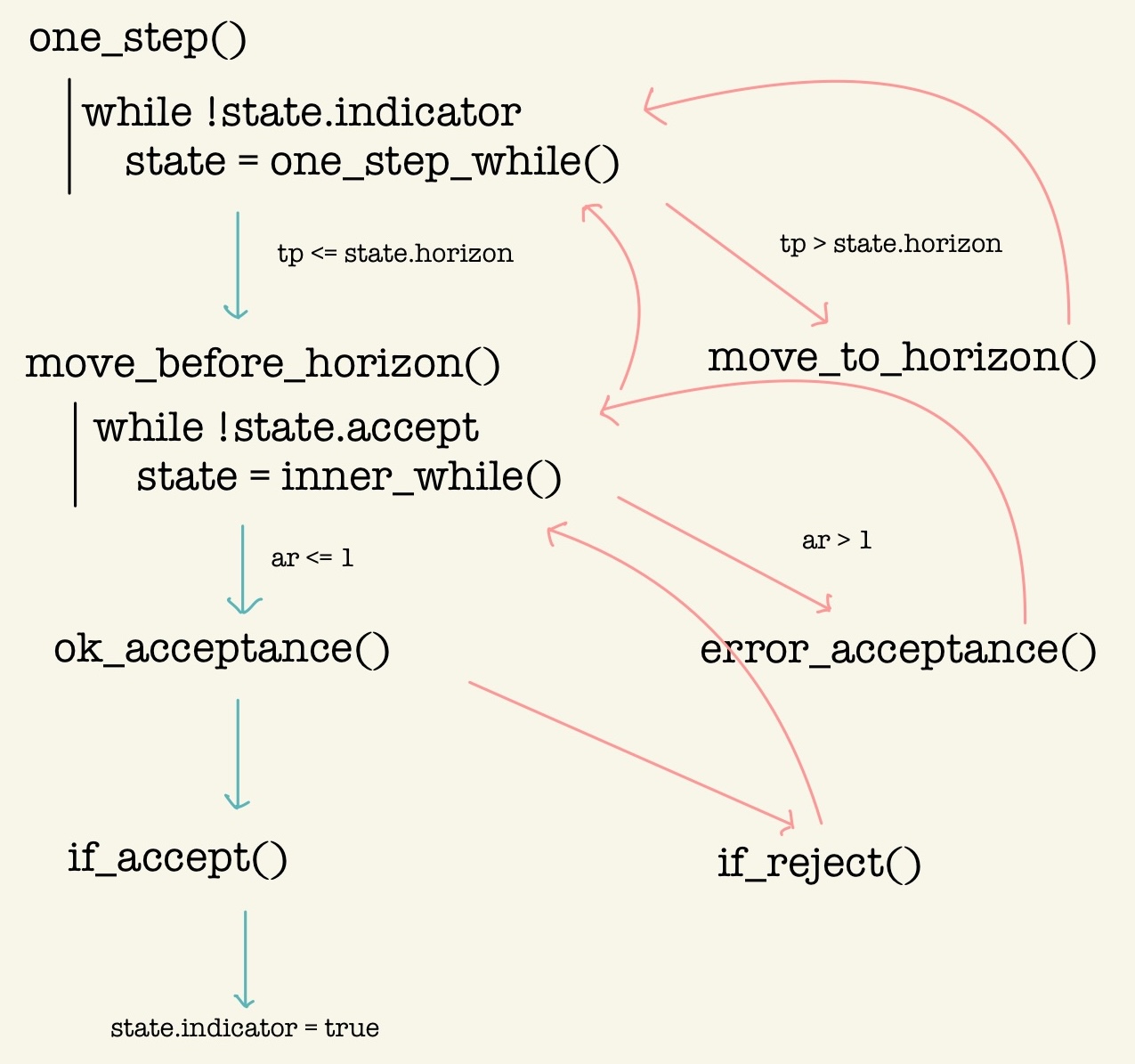
graph TD;
  A["one_step()"] -->|state.indicator=false| B["one_step_while()"]
  B --> C{tp <= state.horizon}
    C -->|No| D[move_to_horizon]
    C -->|Yes| E[move_before_horizon]
    E -->|state.accept=false| G[inner_while]
    G --> I{ar <= 1.0}
    I -->|No| J[error_acceptance]
    I -->|Yes| K[ok_acceptance]
    K -->|reject| L["if_reject()"]
    L -->|場合によっては move_to_horizon2| N["inner_while() か one_step_while() まで戻る"]
    K -->|accept| O["if_accept()
    state.indicator=true
    "]
    D --> B
    J -->|horizon を縮める| N

1. ar=lambda_t/state.lambda_bar によって Poisson thinning を行う．

   ただし，lambda_bar とは近似的な上界であり，「最も近い直前の grid 上の点での値」でしかない．当然 lambda_t を超過し得る．そのような場合に error_acceptance() に入る．

2. error_acceptance() に入った場合，horizon を縮めてより慎重に同じ区間を Poisson thinning しなおす．adaptive=true の場合はこのタイミングで horizon を恒久的に縮める．

3. 最後 if_reject() に入った場合，horizon に到達したら one_step_while() まで戻るが，そうでない場合は inner_while() まで戻る実装がなされている．

2.3 適応的なステップサイズ

3 PDMPFlux.jl パッケージ

3.1 デモ

using PDMPFlux

using Random, Distributions, Plots, LaTeXStrings, Zygote, LinearAlgebra

"""
    Funnel distribution for testing. Returns energy and sample functions.
    For reference, see Neal, R. M. (2003). Slice sampling. The Annals of Statistics, 31(3), 705–767.
"""
function funnel(d::Int=10, σ::Float64=3.0, clip_y::Int=11)

    function neg_energy(x::Vector{Float64})
        v = x[1]
        log_density_v = logpdf(Normal(0.0, 3.0), v)
        variance_other = exp(v)
        other_dim = d - 1
        cov_other = I * variance_other
        mean_other = zeros(other_dim)
        log_density_other = logpdf(MvNormal(mean_other, cov_other), x[2:end])
        return - log_density_v - log_density_other
    end

    function sample_data(n_samples::Int)
        # sample from Nd funnel distribution
        y = clamp.(σ * randn(n_samples, 1), -clip_y, clip_y)
        x = randn(n_samples, d - 1) .* exp.(-y / 2)
        return hcat(y, x)
    end

    return neg_energy, sample_data
end

function plot_funnel(d::Int=10, n_samples::Int=10000)
    _, sample_data = funnel(d)
    data = sample_data(n_samples)

    # 最初の2次元を抽出（yとx1）
    y = data[:, 1]
    x1 = data[:, 2]

    # 散布図をプロット
    scatter(y, x1, alpha=0.5, markersize=1, xlabel=L"y", ylabel=L"x_1", 
            title="Funnel Distribution (First Two Dimensions' Ground Truth)", grid=true, legend=false, color="#78C2AD")

    # xlim と ylim を追加
    xlims!(-8, 8)  # x軸の範囲を -8 から 8 に設定
    ylims!(-7, 7)  # y軸の範囲を -7 から 7 に設定
end
plot_funnel()

function run_ZigZag_on_funnel(N_sk::Int=100_000, N::Int=100_000, d::Int=10, verbose::Bool=false)
    U, _ = funnel(d)
    grad_U(x::Vector{Float64}) = gradient(U, x)[1]
    xinit = ones(d)
    vinit = ones(d)
    seed = 2024
    grid_size = 0  # constant bounds
    sampler = ZigZag(d, grad_U, grid_size=grid_size)
    out = sample_skeleton(sampler, N_sk, xinit, vinit, seed=seed, verbose = verbose)
    samples = sample_from_skeleton(sampler, N, out)
    return out, samples
end
output, samples = run_ZigZag_on_funnel()  # ４分かかる

jointplot(samples)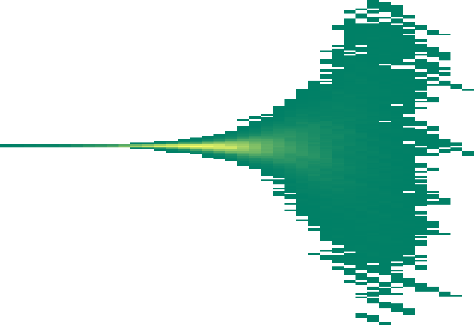

このデモコードは Zygote.jl による自動微分を用いると 5:29 かかっていたところが，ForwardDiff.jl による自動微分を用いると 0:21 に短縮された．

3.2 Zygote.jl と ForwardDiff.jl による自動微分

• JuliaDiff：Differentiation tools in Julia
• Zygote (Docs / GitHub)
• ForwardDiff (Docs / GitHub)

Zygote.jl は FluxML が開発する Julia の自動微分パッケージである．

using Zygote
@time Zygote.gradient(x -> 3x^2 + 2x + 1, 5)

  0.830714 seconds (3.45 M allocations: 168.328 MiB, 3.95% gc time, 99.98% compilation time)

(32.0,)

f(x::Vector{Float64}) = 3x[1]^2 + 2x[2] + 1
g(x) = Zygote.gradient(f,x)
g([1.0,2.0])

([6.0, 2.0],)

大変柔軟な実装を持っており，広い Julia 関数を微分できる．

ForwardDiff.jl (Revels et al., 2016) は Zygote.jl よりも高速な自動微分を特徴としている．

using ForwardDiff
@time ForwardDiff.derivative(x -> 3x^2 + 2x + 1, 5)

  0.068804 seconds (260.59 k allocations: 12.725 MiB, 16.89% gc time, 99.92% compilation time)

32

しかし定義域の次元が \(100\) 以上の場合は ReverseDiff.jl の方が高速になる．

3.3 Brent の最適化

Optim.jl は Julia の最適化パッケージであり，デフォルトで Brent の最適化アルゴリズムを提供する．

using Optim
f(x) = (x-1)^2
result = optimize(f, 0.0, 1.0)
result.minimizer

0.999999984947842

3.4 StatsPlots.jl による可視化

StatsPlots は現在 Plots.jl に統合されている．

また PDMPFlux.jl は marginalhist を wrap した jointplot() 関数を提供する．

3.5 ProgressBars.jl による進捗表示

ProgressBars.jl は tqdm の Julia wrapper を提供する．PDMPFlux.jl ではこちらを採用して，サンプリングの実行進捗を表示する．

なお ProgressMeter.jl も同様の機能を提供しており，有名な別の PDMP パッケージである ZigZagBoomerang.jl ではこちらを採用している．

4 終わりに

今後の確率的プログラミングの１つの焦点は自動微分かもしれない．

今回のパッケージ開発で，少なくとも v0.2.0 の時点では，プログラムに与える U_grad は多くの場合（10 次元の多変量 Gauss，50 次元の Banana など） Zygote.jl が少し速い（Funnel 分布では ForwardDiff.jl が速い）．

しかし上界を構成する際の func の微分は ForwardDiff.jl の方が圧倒的に速い．大変に不可思議である．

だから現在の実装は Zygote.jl と ForwardDiff.jl の両方を用いている．

5 ToDo

• Zig-Zag 以外のサンプラーの実装

• ZigZag(dim) は自動で知ってほしい

• Try clause 内の else を用いているので Julia 1.8 以上が必要．

• MCMCChains のような plot.jl を完成させる．

• PDMPFlux.jl のドキュメントを整備する．

• ZigZagBoomerang.jl を見習って統合したり API をつけたり？

• Turing エコシステムと統合できたりしないか？

• Rng を指定できるようにする？

• pdmp-jax では 37 秒前後かかる Banana density の例が，PDMPFlux.jl では 2 分前後かかる．

  • しかし，Julia の方が数値誤差が少ないのか，banana potential の対称性がうまく結果に出る．尾が消えたりしない．
  • → ForwardDiff.jl を採用したところ，02:05 から 10 分以上に変化した．ReverseDiff.jl を採用したところ 4:44 になった．50 次元というのが微妙なところなのかもしれない．

• Funnel 分布で試したところ，PDMPFlux.jl の棄却率が極めて高い．

6 付録：他に模索した可能性

6.1 Seaborn.jl による可視化

Seaborn.jl は Python の Seaborn の Julia wrapper を提供する．

References

Andral, C., and Kamatani, K. (2024). Automated techniques for efficient sampling of piecewise-deterministic markov processes.

Corbella, A., Spencer, S. E. F., and Roberts, G. O. (2022). Automatic Zig-Zag Sampling in Practice. Statistics and Computing, 32(6), 107.

Neal, R. M. (2003). Slice sampling. The Annals of Statistics, 31(3), 705–767.

Revels, J., Lubin, M., and Papamarkou, T. (2016). Forward-mode automatic differentiation in julia.

Sutton, M., and Fearnhead, P. (2023). Concave-Convex PDMP-based Sampling. Journal of Computational and Graphical Statistics, 32(4), 1425–1435.