Mysteries in Forward Event Chain Monte Carlo

FECMC is a generalization of BPS in that it reduces to BPS (in the limit) when the orthogonal components are fully refreshed.¹

However, an interesting phenomenon is that the scaling limit seems to be entirely different from the BPS case, especially when orthogonal switches are employed as recommended in (Michel et al., 2020).

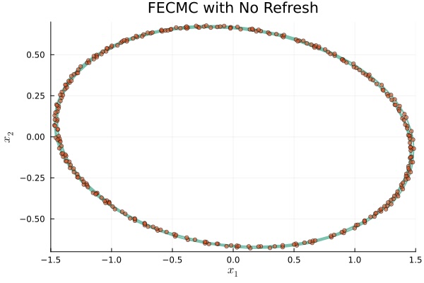
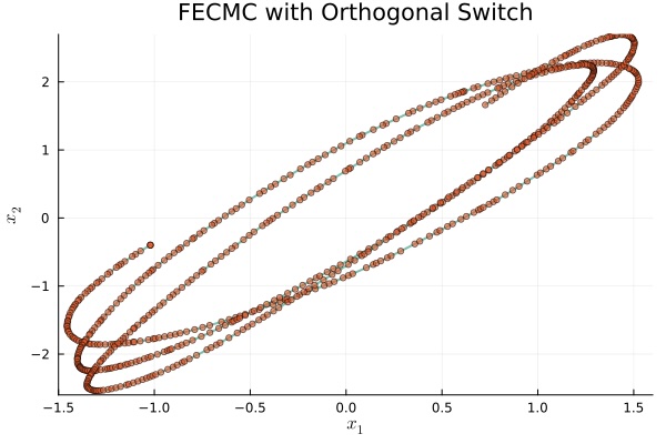
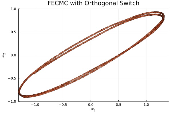
The frequency of orthogonal switches seems to be crucial. As an edge case, without refreshing the orthogonal components, the scaling limit seems to lose ergodicity:

However, the effect of \(p\) decreases as \(d\) increases:

1 Omitted Animations

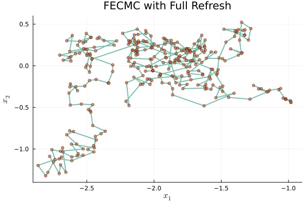
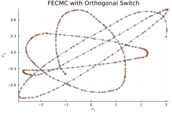
Below we’ll list the animations of the trajectories of FECMC (1) with its orthogonal components fully refreshed, (2) switched, and (3) no orthogonal refresh.

(1) FECMC with its orthogonal components fully refresed

(2) FECMC with its orthogonal components switched

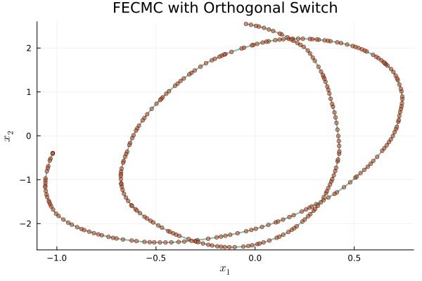
2 The Dynamics of FECMC with no refresh

The deterministic dynamics seems to be determined by the initial value.

Here we add two more examples with different initial values:

3 Diffusion Coefficient Estimation

The diffusion coefficient (denoted by phi) should be \((32/\pi)^{1/4}\approx1.786\), and the drift coefficient (denoted by theta) should be \(\sqrt{2/\pi}\approx0.798\).

When \(d=10^5\) with \(10^6\) skeletons,

Code

library(arrow)

df <- read_feather("FECMC/a.arrow")
library(zoo)
z <- zoo(df$U, order.by = df$t)
library(yuima)
dat <- setData(z)   # yuima.data を作成
dat



Number of original time series: 1
length = 225, time range [0.01 ; 2.25]

Number of zoo time series: 1
         length time.min time.max delta
Series 1    225     0.01     2.25  0.01

Code

df_b <- read_feather("FECMC/b.arrow")
df_b$t <- df_b$t - 0.000025 + df$t[length(df$t)]
df_combined_b <- rbind(df, df_b)
library(zoo)
z <- zoo(df_combined_b$U, order.by = df_combined_b$t)
library(yuima)
dat <- setData(z)

Code

ymodel <- setModel(drift="-theta*x", diffusion="phi")

Warning in yuima.warn("Solution variable (lhs) not specified. Trying to use state variables."): 
YUIMA: Solution variable (lhs) not specified. Trying to use state variables.

Code

param.init <- list(theta=1.0, phi=1.0)
low.par <- list(theta=0.0, phi=0.0)
upp.par <- list(theta=2.0, phi=2.0)
yuima <- setYuima(model=ymodel, data=dat)
mle1 <- qmle(yuima, start=param.init, lower=low.par, upper=upp.par)
summary(mle1)

Quasi-Maximum likelihood estimation

Call:
qmle(yuima = yuima, start = param.init, lower = low.par, upper = upp.par)

Coefficients:
      Estimate Std. Error
phi   1.751459 0.05858751
theta 1.783468 0.88841968

-2 log L: -290.3644

Code

df_c <- read_feather("FECMC/c.arrow")
df_c$t <- df_c$t - 0.0000224 + df$t[length(df$t)]
df_combined_c <- rbind(df, df_c)
library(zoo)
z <- zoo(df_combined_c$U, order.by = df_combined_c$t)
library(yuima)
dat <- setData(z)

Code

ymodel <- setModel(drift="-theta*x", diffusion="phi")

Warning in yuima.warn("Solution variable (lhs) not specified. Trying to use state variables."): 
YUIMA: Solution variable (lhs) not specified. Trying to use state variables.

Code

param.init <- list(theta=1.0, phi=1.0)
low.par <- list(theta=0.0, phi=0.0)
upp.par <- list(theta=2.0, phi=2.0)
yuima <- setYuima(model=ymodel, data=dat)
mle1 <- qmle(yuima, start=param.init, lower=low.par, upper=upp.par)
summary(mle1)

Quasi-Maximum likelihood estimation

Call:
qmle(yuima = yuima, start = param.init, lower = low.par, upper = upp.par)

Coefficients:
      Estimate Std. Error
phi   1.674266 0.04662068
theta 1.922156 0.76559726

-2 log L: -477.9923

References

Michel, M., Durmus, A., and Sénécal, S. (2020). Forward event-chain monte carlo: Fast sampling by randomness control in irreversible markov chains. Journal of Computational and Graphical Statistics, 29(4), 689–702.

Footnotes

FECMC with full orthogonal refresh is \(d\to\infty\) asymptotically equivalent to BPS, allegedly.↩︎