High-Dimensional Behaviour of Piecewise Deterministic Monte Carlo

Today’s Contents

Section 1 What is PDMP?

→ A new class of continuous-time Monte Carlo methods
Section 2 High-Dimensional Scaling Analysis

→ FECMC always performs better than BPS
Section 3 Asymptotic Variance / ESS Estimation

→ PDMP algorithms allow a more efficient estimator

1 PDMPs: A New Frontier of Monte Carlo

Let me start by placing PDMP in the broader history of Monte Carlo methods. The history starts with a Markov chain driven by a simple uniform random variable, originally simulated on the MANIAC computer (Metropolis et al., 1953). Then the attention naturally shifted to more structured stochastic processes, such as Langevin diffusion (Rossky et al., 1978) and PDMP (Michel et al., 2014), (Peters and de With, 2012).

1.1 PDMP: Mathematical Definition

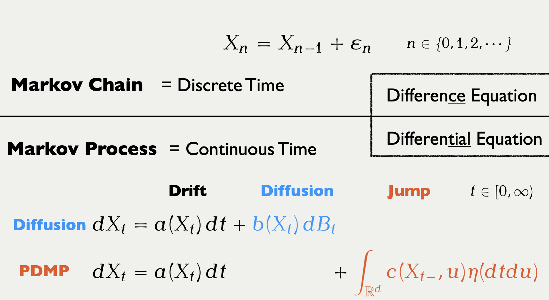
PDMP is a class of Markov processes that complements the diffusion process. A PDMP is a `diffusion’ process driven by jumps, rather than a Brownian motion. An important consequence is a strong ballistic / transport property, which is typically absent in a Langevin diffusion. Informally, the Brownian term moves only on the scale of \Delta B_t \sim \sqrt{\Delta t}.

1.2 Markov Chain Monte Carlo

These processes are routinely used in the MCMC methodologies. However, notice that the trajectory of Langevin diffusion requires a discretization, while the output of PDMP potentially allows sparse representations, by retaining the event-time information and the new velocity at these points.

1.3 Classical Methods Turn Out to Be PDMPs in Disguise

Many PDMPs behave similarly in high dimensions.

discretized by a symplectic integrator

e.g. HMC has O(d^{1.25}) complexity

simulate piecewise linear trajectory

e.g. BPS with normal velocity has O(d^{1.5}) complexity

So far, I may have suggested that PDMP is an entirely new class of MCMC methods. Yes, in some sense, e.g., the output is a continuous trajectory instead of a set of discrete samples. However, though the term may be new to the field, it might be nothing new conceptually. To me, PDMP also works as an umbrella term that helps shed light upon a previously overlooked aspect of classical MCMC methods.

This is a somewhat strong claim, but let me pose it this way. Somehow, every successful MCMC method is implicitly a PDMP. To be precise, it chases Hamiltonian dynamics in high-dimensional settings, which may be one of the reasons why PDMP is a class of Markov processes worth considering collectively (Deligiannidis et al., 2021).

The randomized Hamiltonian Monte Carlo dynamics mix fast regardless of the dimension (for a certain class of target). From this point of view, classical Hamiltonian Monte Carlo and Bouncy Particle Sampler give different ways of numerically simulating the same dynamics.

We see a trade-off between the computational complexity and the robustness of the method.

1.4 Digression: Killer Applications of PDMP

x: CPU time, y: Estimate．(Bouchard-Côté et al., 2018)
Sparse Markov Random Field with d=10

O(d^1) Local Implementation

Exploiting sparsity, BPS atteins better scaling than HMC (MSE/sec.)

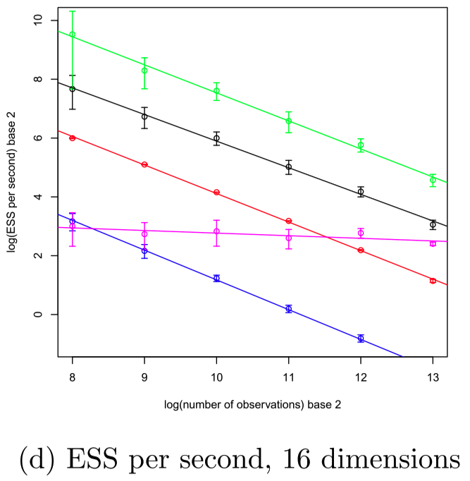
Stochastic Gradient O(n^0)

x: sample size n, y: log ESS
Logistic regression with d=16
Using an appropriate control variate, the efficiency of Zig-Zag is O(1)
in the limit of n\to\infty, it outperforms Langevin.

I briefly touch upon some killer applications of PDMP, as they are important motivations for the development of PDMP.

2 Towards Better Jump Strategy: A Scaling Analysis

We compare two famous PDMP methods under the following condition:

ODE: Fixed
Jump: Reflection + Refreshment vs. Combination
Target: High dimensional standard Gaussian U(x):=-\log\pi(x)=\|x\|^2/2.

2.1 BPS vs. FECMC

Bouncy Particle Sampler (Bouchard-Côté et al., 2018)

Forward Event Chain Monte Carlo (Michel et al., 2020)

To get straight to the point, we compare the two methods with possibly different hyperparameter values \rho. Once animated, one might easily see the red method, Forward Event-Chain Monte Carlo proposed in (Michel et al., 2020), is the fastest. We would like to show this quantitatively, together with dependence upon \rho.

2.2 Jump Strategy in BPS vs. FECMC

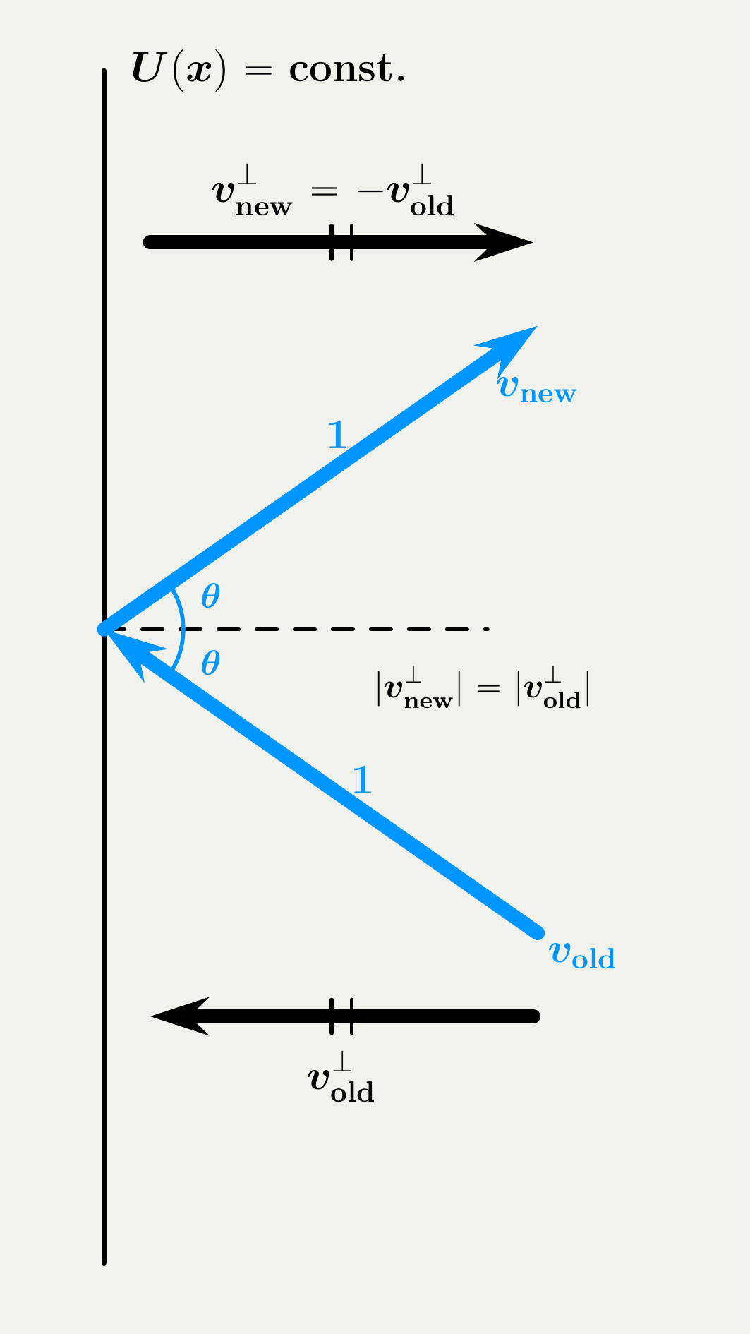
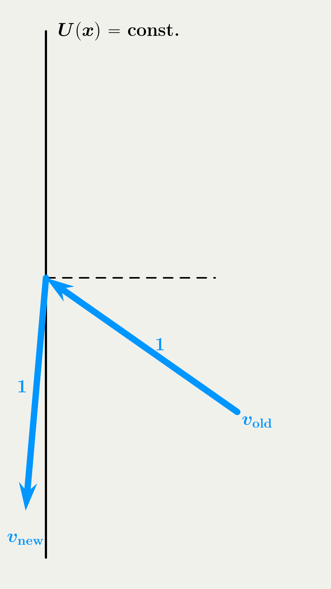
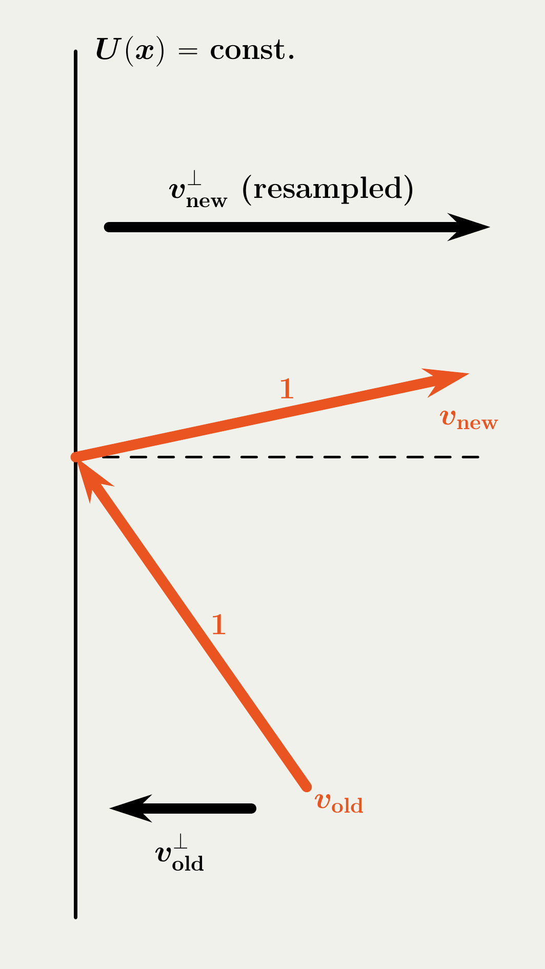
The velocity jump mechanism in BPS is simpler and we start with it. When jumps, the BPS process either reflect or refresh. On reflection, the process changes the velocity as a light ray does, matching the incidence and reflection angles. On refreshment, the process resamples the velocity from the invariant distribution, a uniform distribution on the unit sphere in our setting.

Forward Event-Chain Monte Carlo, on the other hand, is more sophisticated, combining the two mechanisms.

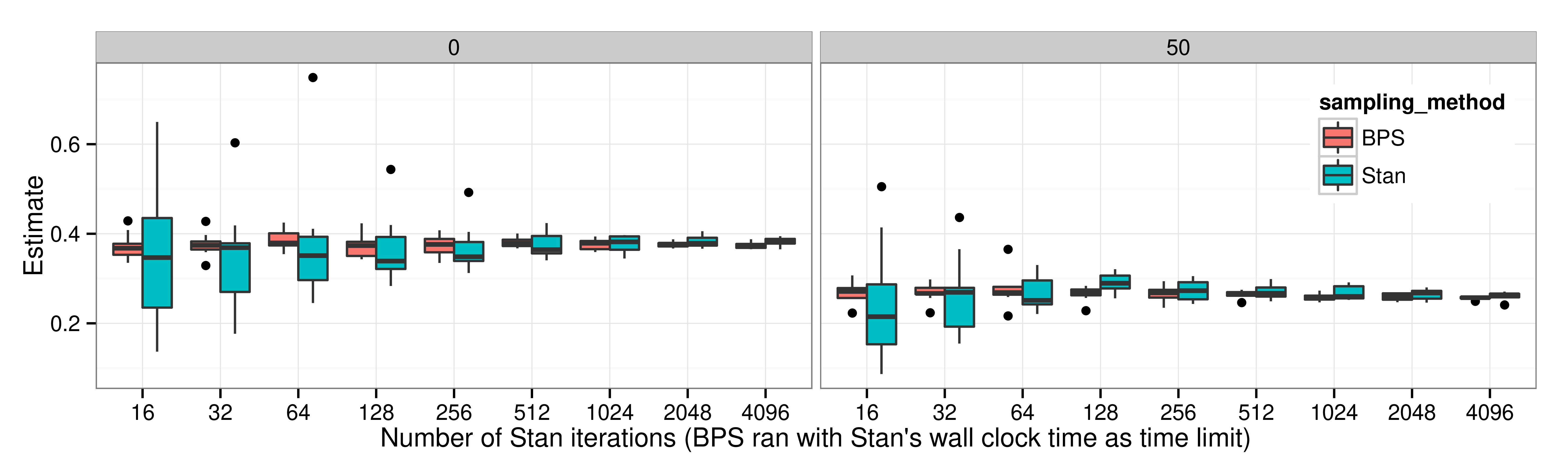
2.3 Empirical Comparison: BPS vs. FECMC

Effective Sample Size of U(x)=\|x\|^2, the negative log-density of 100 dimensional standard Gaussian, estimated over 1000 runs

2.4 Scaling Analysis = Deriving a Diffusion Limit

\text{Plotting } \textcolor{#0096FF}{Y_t^{(d)}}=\frac{\lvert\textcolor{#0096FF}{X}_{d\textcolor{#0096FF}{t}}^{\textcolor{#0096FF}{(d)}}\rvert^2-d}{\sqrt{d}} \text{ with } d=10^2,10^3,10^4:

2.5 Theorem 1： Diffusion Limits of FECMC & BPS

dY_t^{\textcolor{#0096FF}{\text{B}}}=-\frac{\sigma^2_{\textcolor{#0096FF}{\text{B}}}(\rho)}{4}Y_t^{\textcolor{#0096FF}{\text{B}}}\,dt+\sigma_{\textcolor{#0096FF}{\text{B}}}(\rho)\,dB_t \sigma^2_{\textcolor{#0096FF}{\text{B}}}(\rho)=8\int^\infty_0e^{-\rho s}\operatorname{E}[R_0^{\textcolor{#0096FF}{\text{B}}}R_s^{\textcolor{#0096FF}{\text{B}}}]\,ds

dY_t^{\textcolor{#E95420}{\text{F}}}=-\frac{\sigma^2_{\textcolor{#E95420}{\text{F}}}(\rho)}{4}Y_t^{\textcolor{#E95420}{\text{F}}}\,dt+\sigma_{\textcolor{#E95420}{\text{F}}}(\rho)\,dB_t \sigma^2_{\textcolor{#E95420}{\text{F}}}(\rho)=8\int^\infty_0e^{-\rho s}\operatorname{E}[R_0^{\textcolor{#E95420}{\text{F}}}R_s^{\textcolor{#E95420}{\text{F}}}]\,ds

2.6 Theorem 2: Analytic Expression of \sigma^2’s

While BPS atteins maximum at non-trivial value of \rho, FECMC achieves maximum at \rho=0

2.7 Sketch of Proof: the non-Markovianity of Y^d

Doob-Meyer Decomposition (Doléans-Dade and Meyer, 1970 Theorem 4)

Y^d is non-Markovian, but is a (special) semimartingale, having Y^d_t=Y^d_0+B^d_t+M^d_t, where B^d is the dual predictable projection of Y^d, and M^d is a local L^2-martingale.

Convergence of Semimartingales (Jacod and Shiryaev, 2003 Theorem IX.3.48)

The convergence of B^d and C^d_t:=\langle M^d\rangle_t (in a suitable sense) to B_t=-\int^t_0\frac{\sigma^2}{4}Y_s\,ds,\quad C_t=\sigma^2t, is one of the sufficient conditions of the weak convergence Y^d\Rightarrow Y when dY_t=-\frac{\sigma^2}{4}Y_t\,dt+\sigma\,dB_t.

2.8 Asymptotic Equivalence to a Skeleton Process

Original Potential Process \textcolor{#0096FF}{Y^d}

B^d_t=2\sqrt{d}\int^t_0R^d_{ds-}\,ds,%\quad R_t^d:=\brac{X_t^d,V_t^d}, C^d_t=0.

Difficult to see how C_t=\sigma^2t emerges.

Event-Time Skeleton \textcolor{#0096FF}{\overline{Y}^d}

\overline{B}^d_t=\sum_{n=1}^{N_t}\operatorname{E}[\Delta\overline{Y}^d_n|\overline{\mathcal{F}}^d_{n-1}] {\scriptsize \overline{C}^d_t=\sum_{n=1}^{N_t}\left(\operatorname{E}[(\Delta\overline{Y}^d_n)^2|\overline{\mathcal{F}}^d_{n-1}]-\operatorname{E}[\Delta\overline{Y}^d_n|\overline{\mathcal{F}}^d_{n-1}]^2\right).}

3 Asymptotic Variance / ESS Estimation for PDMP (or continuous-time MCMC more broadly)

There is a fundamental difference between the Monte Carlo estimators produced by

\text{PDMP}\quad\widehat{h}_T^{\textcolor{#E95420}{\text{PDMP}}}=\frac{1}{T}\int^T_0h(\textcolor{#E95420}{X}_{\textcolor{#E95420}{t}}^{\textcolor{#E95420}{(d)}})\,dt,\quad t\in[0,T], \text{classical MCMC}\quad\widehat{h}_N^{\textcolor{#0096FF}{\text{MCMC}}}=\frac{1}{N}\sum_{n=1}^Nh(\textcolor{#0096FF}{X_n^{(d)}}),\quad n=1,\cdots,N.

Exploiting this continuous-time nature of PDMP, we can introduce more efficient estimators for the asymptotic variance of \widehat{h}_T^{\textcolor{#E95420}{\text{PDMP}}}.

Algorithmically, there is a fundamental difference in the Monte Carlo estimator produced by PDMP & classical MCMC. As the algorithm outputs a continuous trajectory, we are able to look into fine structure of the trajectory, which is not possible with classical MCMC.

3.1 Implications of the Diffusion Limit Results

Corollary (Relationship between \sigma^2 and ESS)

The effective sample size (ESS) for estimating U with a trajectory of length \textcolor{#E95420}{d}T is given by \operatorname{ESS}(U)\fallingdotseq\frac{\sigma^2}{8}T\qquad(d\to\infty).

[Proof] The Monte Carlo estimator (= ergodic average of \textcolor{#E95420}{\{X_t\}}) \widehat{h}_T^d:=\frac{1}{T}\int^T_0U(\textcolor{#E95420}{X_t^{(d)}})\,dt has a computable variance under double asymptotic limit: \lim_{T\to\infty}\lim_{d\to\infty}T\frac{\operatorname{Var}[\widehat{h}_{\textcolor{#E95420}{d}T}^d]}{\operatorname{Var}_\pi[U]}=\frac{8}{\sigma^2}\approx2.50\cdots. ESS equals the inverse of this variance ratio.

3.2 Theory Matches Practice: FECMC vs. BPS

ESS for U estimated over 1000 runs. Every bootstrap CI contains the theoretical limiting value {8}/{\sigma^2}.

3.3 Asymptotic Variance Estimation for MCMC

A practical issue: Does this trajectory suffice for mean estimation? → A solution: asymptotic variance estimation

\text{Markov Chain CLT: }\quad\frac{1}{\sqrt{N}}\sum_{n=1}^NX_n\Rightarrow N(0,\sigma^2_{\text{asym}})\quad(N\to\infty). For mini-batches b=1,\cdots,B with length m:=N/B, \operatorname*{{Batch\; Means\; Estimator:}}_{\text{(for mean estimation)}} \text{ }\quad\widehat{\sigma^2}_\text{asym}:=\frac{m}{B-1}\sum_{b=1}^B\left(\textcolor{#0096FF}{\overline{{X}}^{(b)}}-\textcolor{#0096FF}{\overline{{X}}}\right)^2, where \textcolor{#0096FF}{\overline{{X}}^{(b)}}=\frac{1}{m}\sum_{n=1}^m\textcolor{#0096FF}{X_{n+(b-1)m}} is the mean over the b-th batch.

3.4 Optimal Batch Size for Classical MCMC & PDMP

Due to the continuous-time nature, batch size selection becomes a nontrivial problem for PDMPs.

MSE Minimizing Batch Size for Classical MCMC (Liu et al., 2022)

m_{\text{opt}}=\left(\frac{\gamma_{\text{disc}}}{\sigma_{\text{asym}}^2}\right)^{\frac{2}{3}}N^{\frac{1}{3}} minimizes the MSE asymptotically under m\to\infty,\qquad N/m\to\infty, for a sufficiently mixing Markov chain \{\textcolor{#0096FF}{X_n}\}.

Bias Minimizing Batch Size for PDMP (S. & Kamatani 2026+)

Analogously, with \gamma_{\text{disc}}=2\sum_{k=0}^\infty k\operatorname{Cov}[\textcolor{#0096FF}{X_0},\textcolor{#0096FF}{X_k}] replaced by \gamma_{\text{cont}}=2\int^\infty_0t\operatorname{Cov}[\textcolor{#E95420}{X_0},\textcolor{#E95420}{X_t}]\,dt.

3.5 Diffusivity Estimation for High-dimensional PDMPs

= Quadratic Variation (QV) Estimation under Misspecification

Plot of Y_t^d:=(|\textcolor{#E95420}{X^d}_{d\textcolor{#E95420}{t}}|^2-d)/\sqrt{d} when d=10^4. The trajectory converges to dY_t=-\frac{\sigma^2}{4} Y_t\,dt+\sigma\,dB_t as d\to\infty

The Realized Volatility estimator (Barndorff-Nielsen and Shephard, 2002) \widehat{Q}^d:=\frac{1}{T}\sum_{n=1}^N\biggr(Y_{\Delta n}^d-Y_{\Delta(n-1)}^d\biggl)^2,\quad T=\Delta N, converges to \sigma^2 under the conditions \Delta\to0,\quad d\to\infty,\quad\Delta d\to\infty.

3.6 Experiment: QV Estimation Improves with Dimension

slow corresponds to the Batch Means estimator, fast corresponds to the Realized Variation estimator

3.6 Experiment: QV Estimation Improves with Dimension

slow corresponds to the Batch Means estimator, fast corresponds to the Realized Variation estimator

3.7 Batch Size Selection for the QV Estimator

\fallingdotseq selecting the sampling step size \Delta under Misspecification (Aït-Sahalia et al., 2011)

Plot of Y_t^d:=(|\textcolor{#E95420}{X^d}_{d\textcolor{#E95420}{t}}|^2-d)/\sqrt{d} when d=10^4. Taking a closer look, the trajectory is an ODE, a `microstructure noise’

For too small / large \Delta, \widehat{Q}^{d}(\Delta)\approx0. The optimal choice seems to be \Delta=O(d^{1/2}).

Conclusion

Reducing redundant noise produces a more efficient algorithm: BPS → FECMC
Continuous-time MCMC allows more efficient estimators for asymptotic variance
- potentially works whenever a diffusion limit exists

References

Aït-Sahalia, Y., Mykland, P. A., and Zhang, L. (2011). Ultra High Frequency Volatility Estimation with Dependent Microstructure Noise. Journal of Econometrics, 160(1), 160–175.

Barndorff-Nielsen, O. E., and Shephard, N. (2002). Estimating Quadratic Variation using Realized Variance. Journal of Applied Econometrics, 17(5), 457–477.

Bierkens, J., Fearnhead, P., and Roberts, G. (2019). The Zig-Zag Process and Super-Efficient Sampling for Bayesian Analysis of Big Data. The Annals of Statistics, 47(3), 1288–1320.

Bouchard-Côté, A., Vollmer, S. J., and Doucet, A. (2018). The Bouncy Particle Sampler: A Nonreversible Rejection-Free Markov Chain Monte Carlo Method. Journal of the American Statistical Association, 113(522), 855–867.

Deligiannidis, G., Paulin, D., Bouchard-Côté, A., and Doucet, A. (2021). Randomized Hamiltonian Monte Carlo as scaling limit of the bouncy particle sampler and dimension-free convergence rates. The Annals of Applied Probability, 31(6), 2612–2662.

Doléans-Dade, C., and Meyer, P.-A. (1970). Intégrales Stochastiques par Rapport aux Martingales Locales. Séminaire de Probabilités, 4, 77–107.

Jacod, J., and Shiryaev, A. N. (2003). Limit Theorems for Stochastic Processes,Vol. 288. Springer Berlin, Heidelberg.

Liu, Y., Vats, D., and Flegal, J. M. (2022). Batch Size Selection for Variance Estimators in MCMC. Methodology and Computing in Applied Probability, 24(1), 65–93.

Metropolis, N., Rosenbluth, A. W., Rosenbluth, M. N., Teller, A. H., and Teller, E. (1953). Equation of state calculations by fast computing machines. The Journal of Chemical Physics, 21(6), 1087–1092.

Michel, M., Durmus, A., and Sénécal, S. (2020). Forward Event-Chain Monte Carlo: Fast Sampling by Randomness Control in Irreversible Markov Chains. Journal of Computational and Graphical Statistics, 29(4), 689–702.

Michel, M., Kapfer, S. C., and Krauth, W. (2014). Generalized event-chain monte carlo: Constructing rejection-free global-balance algorithms from infinitesimal steps. The Journal of Chemical Physics, 140(5), 054116.

Peters, E. A. J. F., and de With, G. (2012). Rejection-free monte carlo sampling for general potentials. Physical Review E, 85(2).

Rossky, P. J., Doll, J. D., and Friedman, H. L. (1978). Brownian dynamics as smart Monte Carlo simulation. The Journal of Chemical Physics, 69(10), 4628–4633.