High-Dimensional Behaviour of Two Piecewise Deterministic Markov Processes

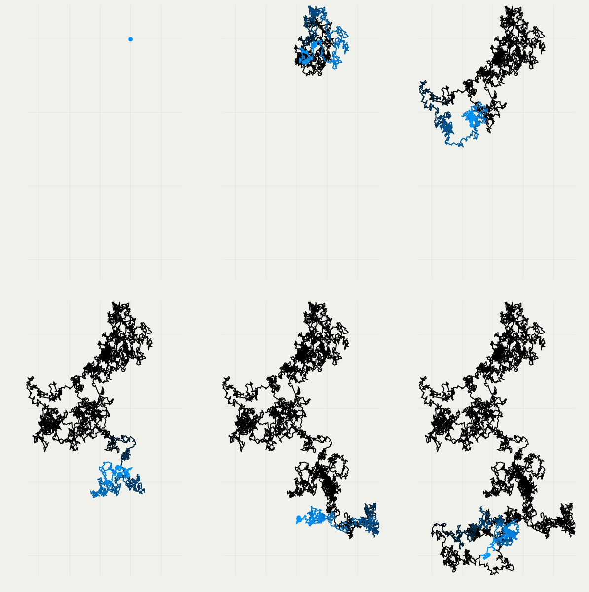
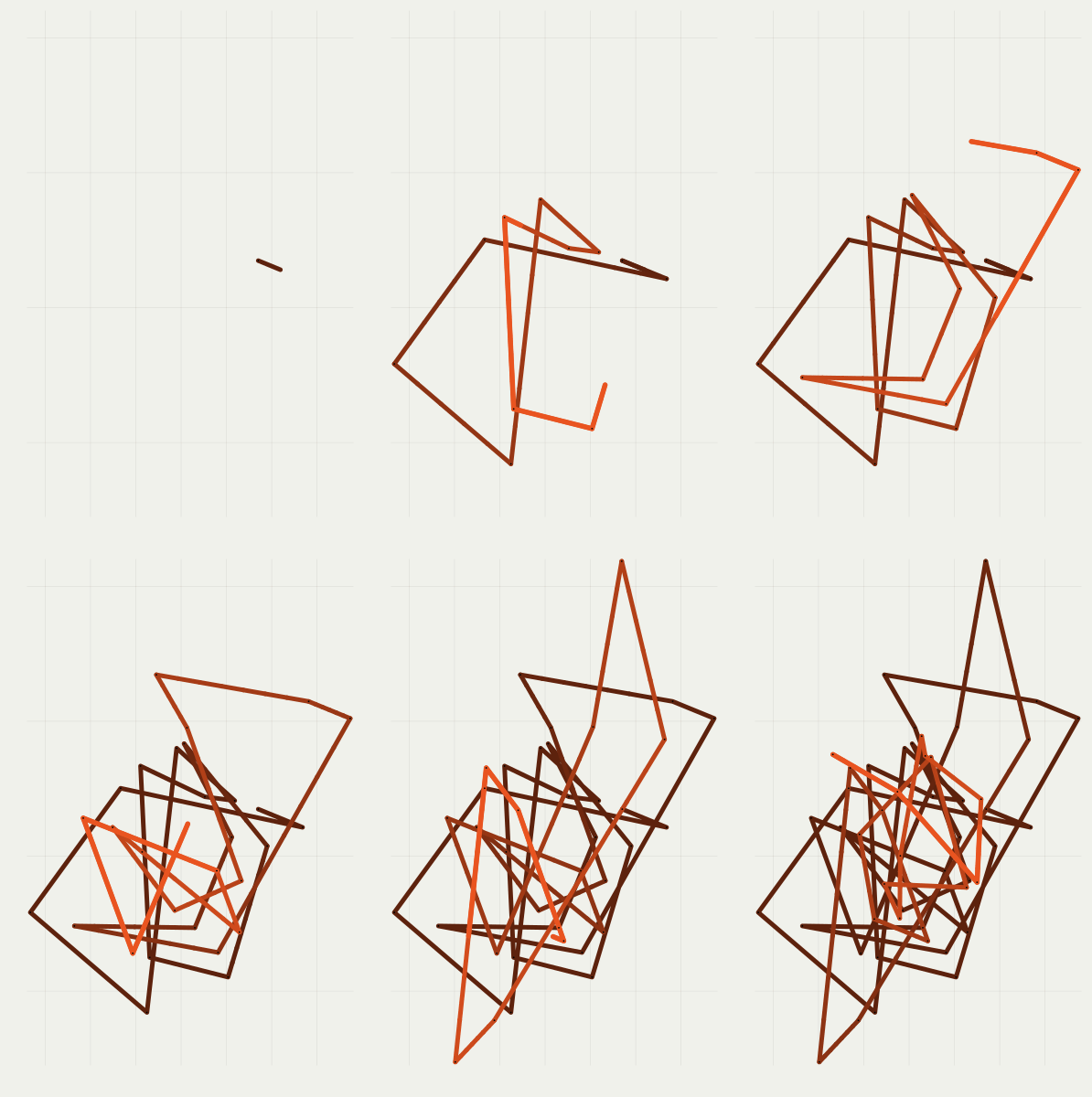
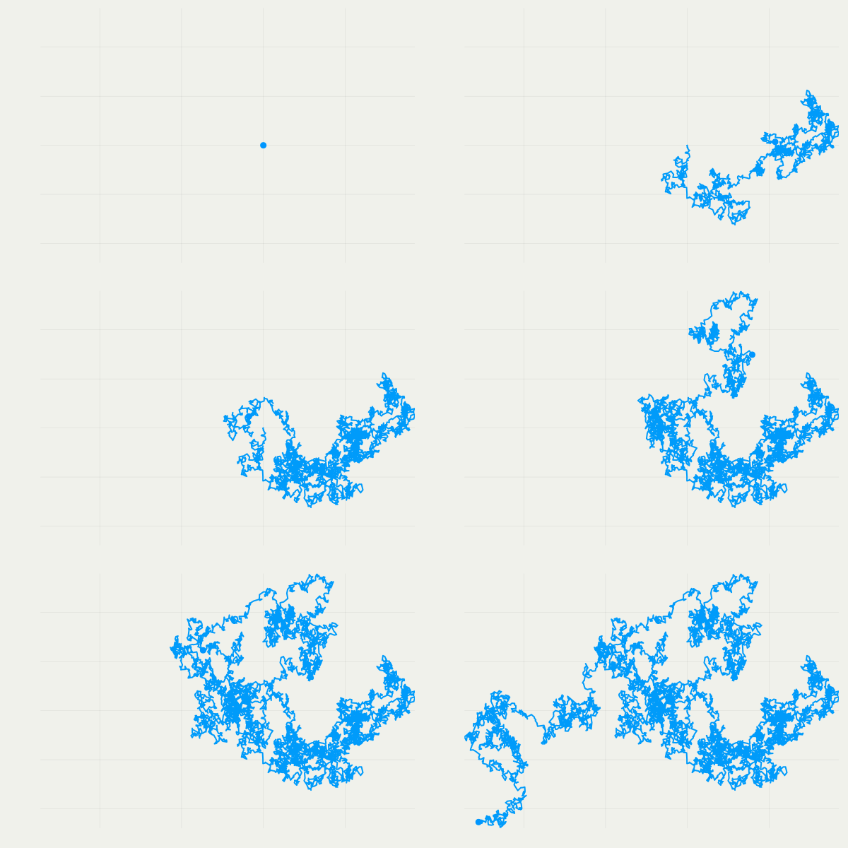
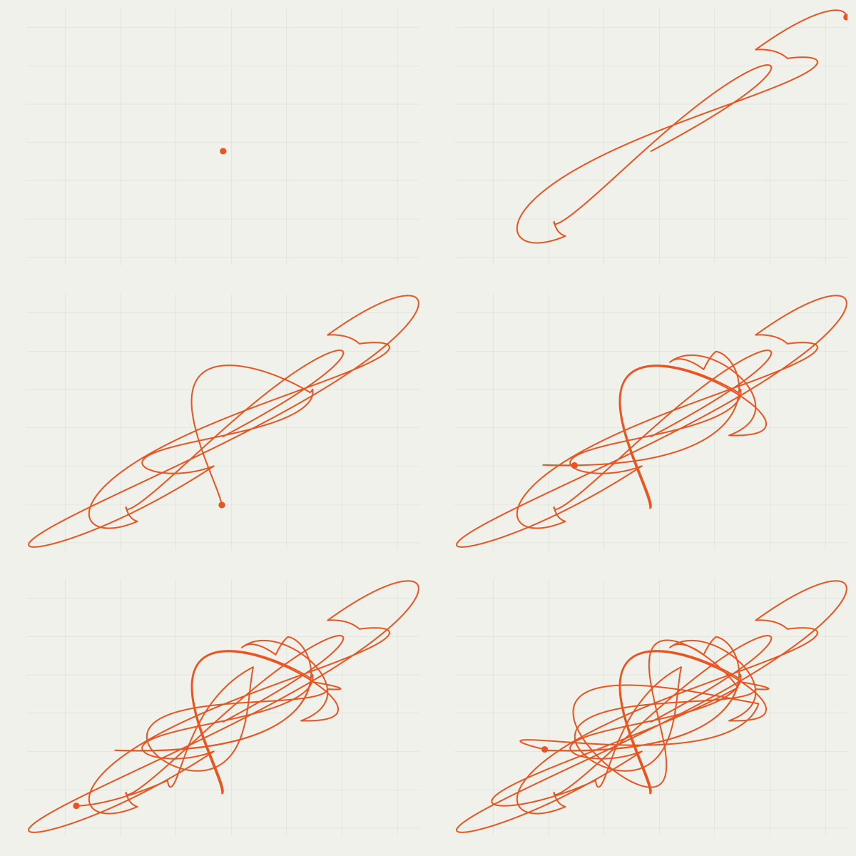
Efficiency Comparison & Asymptotic Variance Estimation

Hirofumi Shiba

Institute of Statistical Mathematics, Tokyo, Japan

10/13/2026

Scaling Analysis of Two PDMPs

  • Section 1: \;What is PDMP?

    A new class of continuous-time Monte Carlo dynamics

  • Section 2: \;What is scaling analysis?

    FECMC always performs better than BPS

  • Section 3: \;Proof Strategy

  • Section 4: \;Asymptotic variance estimation (≒ ESS estimation)

    The PDMP framework allow a more efficient estimator

1 PDMP: A New Frontier of Monte Carlo

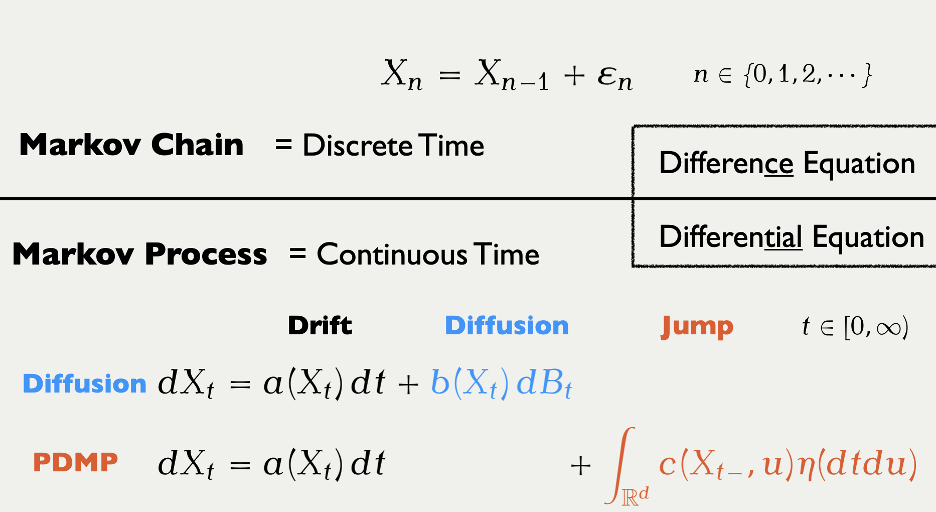
Markov Chain
(1953–)

Langevin Diffusion
(1978–)

PDMP
(2008–)

1.1 Piecewise-Deterministic Markov Process
Langevin Diffusion

Randomized Hamiltonian Monte Carlo

1.2 Markov Chain Monte Carlo

computes space averages as time averages
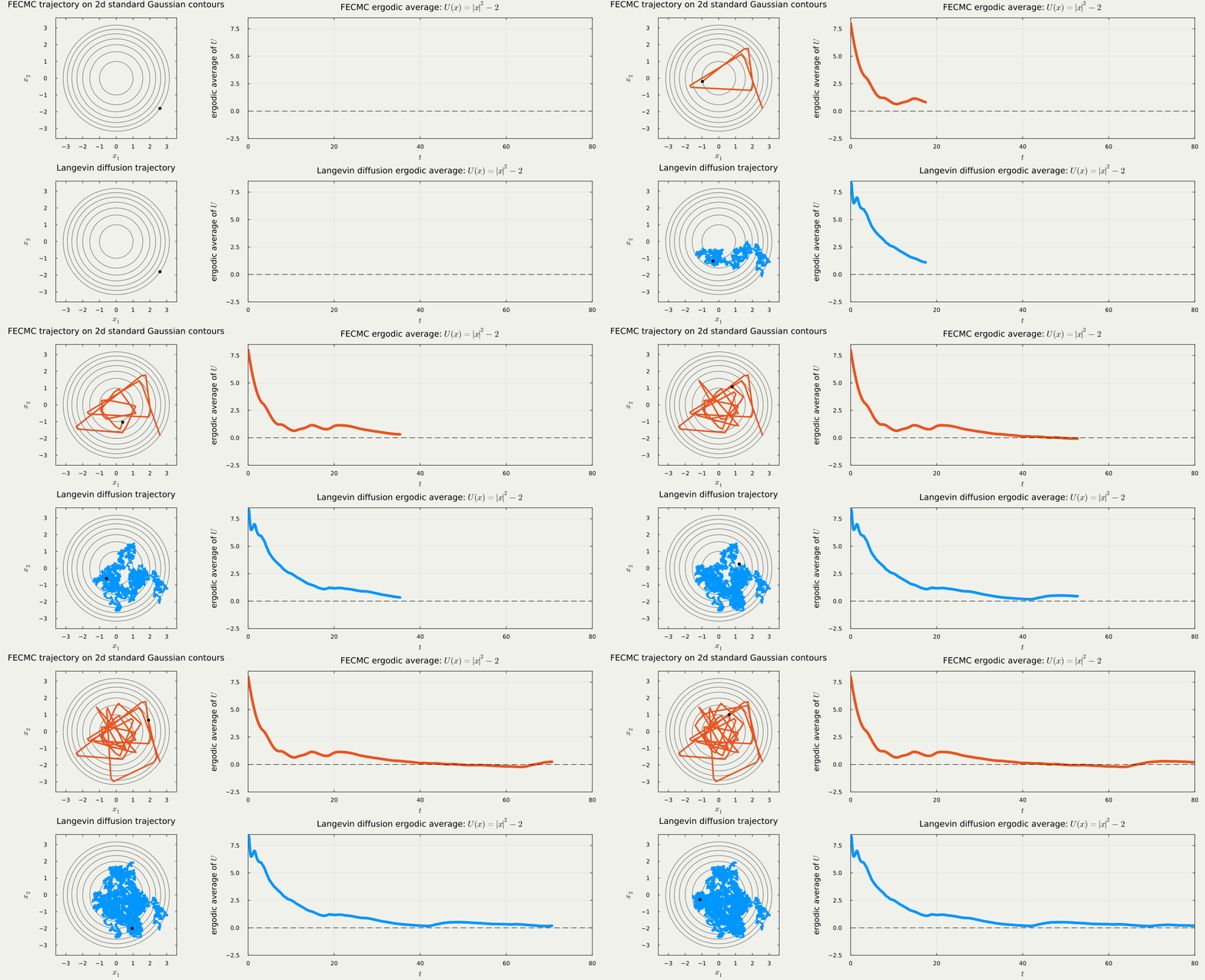
1.3 Persistent Exploration with Hypocoercivity

Underdamped Langevin

Kinetic Langevin

\begin{cases} \dot{X}_t=V_t,\\ \dot{V}_t=-\big(\nabla U(X_t)-\gamma V_t\big)\,dt+\sqrt{2\gamma}\,dB_t. \end{cases}

Forward Event-Chain Monte Carlo

Velocity-Jump PDMP

\begin{cases} \dot{X}_t=V_{t-},\\ \dot{V}_t=\big(\operatorname{Jump}_{X_t}(V_{t-};\xi_t)-V_{t-}\big)\,dN_t. \end{cases}

1.4 PDMP as a New Discretisation Scheme

Many PDMP and MCMC behave similarly in high dimensions (Deligiannidis et al., 2021)
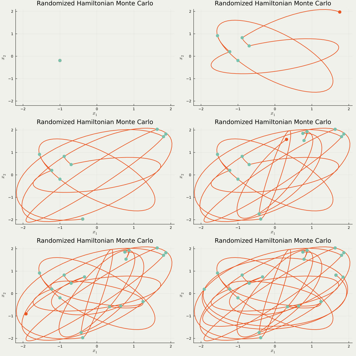
RHMC (d=2)

discretized by a symplectic integrator

e.g. HMC has O(d^{1.25}) complexity
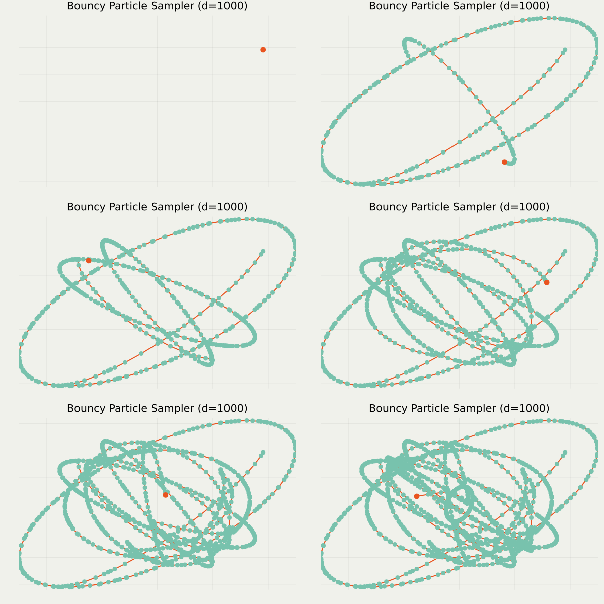
BPS with Gaussian speed (d=10^3)

simulate piecewise linear trajectory

e.g. BPS with normal velocity has O(d^{1.5}) complexity

1.5 In Passing… Some Killer Applications of PDMP
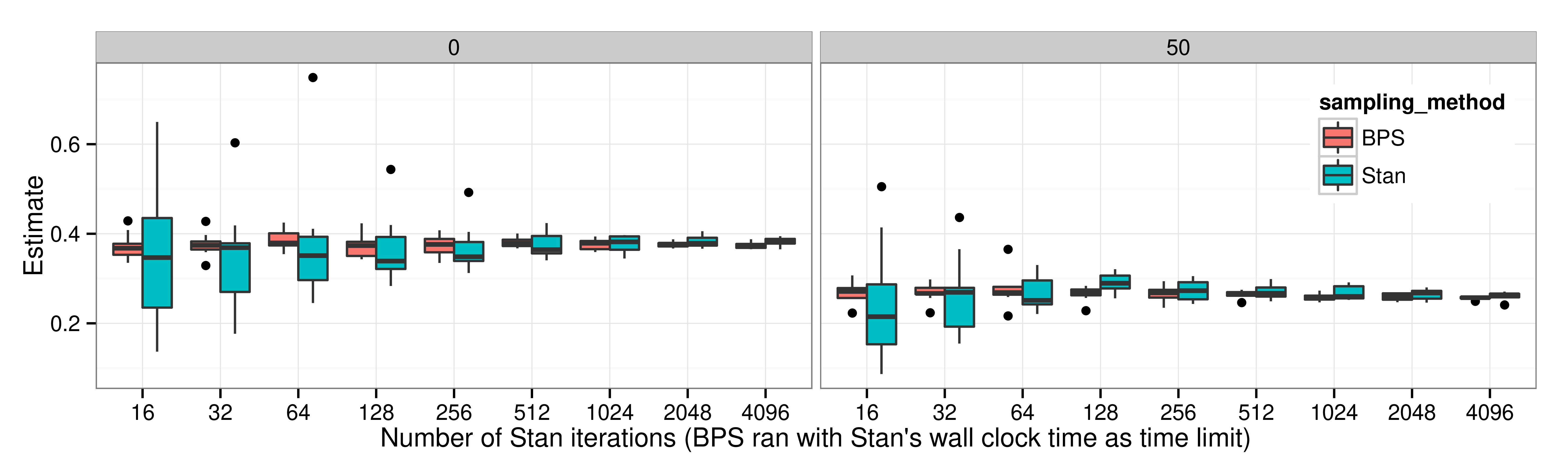
x: CPU time, y: Estimate.(Bouchard-Côté et al., 2018)
Sparse Markov Random Field with d=10

O(d^1) Local Implementation

Exploiting sparsity, BPS atteins better scaling than HMC (MSE/sec.)
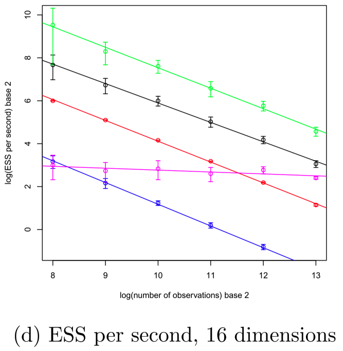
x: sample size n, y: log ESS/sec, d=16
(Bierkens et al., 2019)

Stochastic Gradient O(n^0)

Using an appropriate control variate, Zig-Zag attains O(1) complexity
in the limit of n\to\infty, it outperforms Langevin.

2 A Scaling Analysis

We compare two famous PDMP methods under the following condition:

  • ODE: Fixed
  • Jump: Reflection + Refreshment vs. Combination
  • Target: High dimensional standard Gaussian U(x):=-\log\pi(x)=\|x\|^2/2.

2.1 BPS vs. FECMC: Which is Most Efficient?
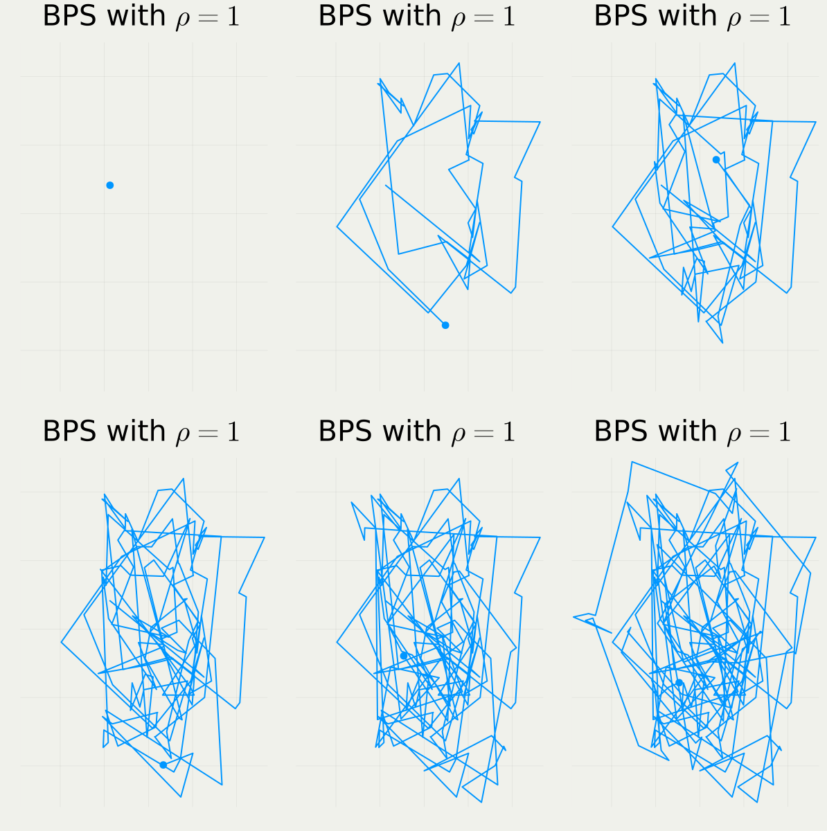
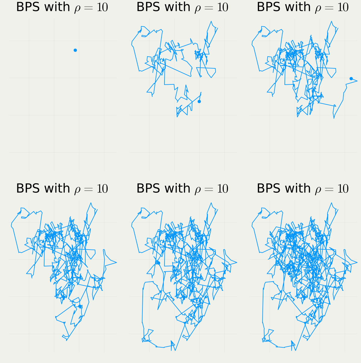
Bouncy Particle Sampler
(Bouchard-Côté et al., 2018)

BPS with different hyperparameter \rho

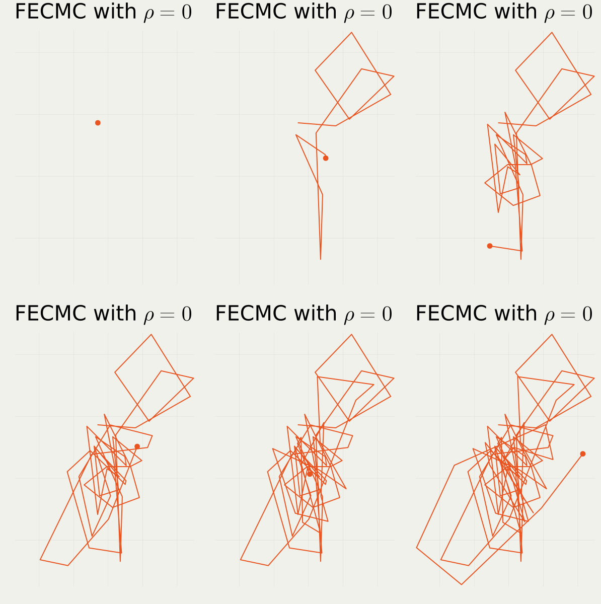
Forward Event Chain Monte Carlo (Michel et al., 2020)

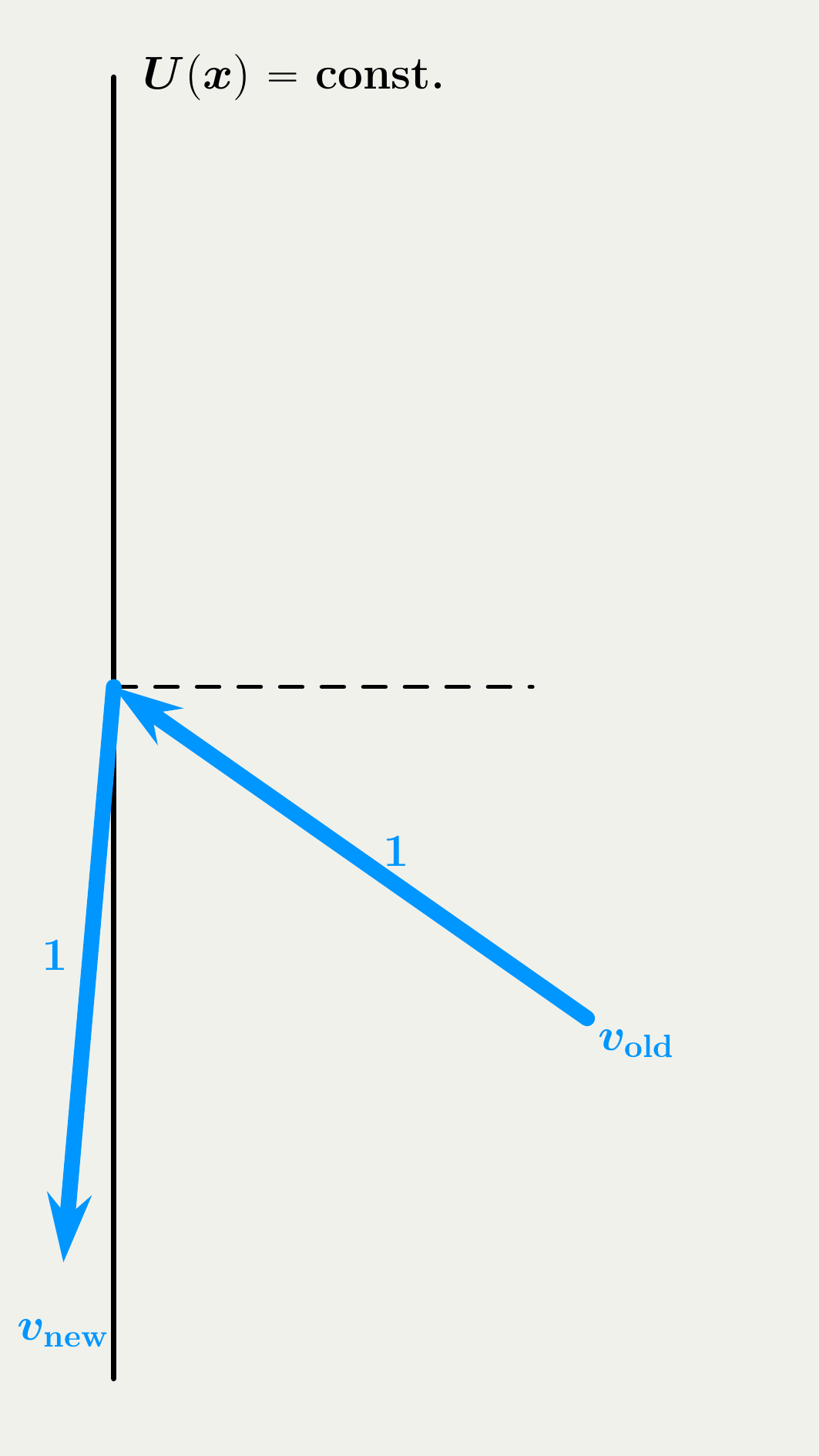
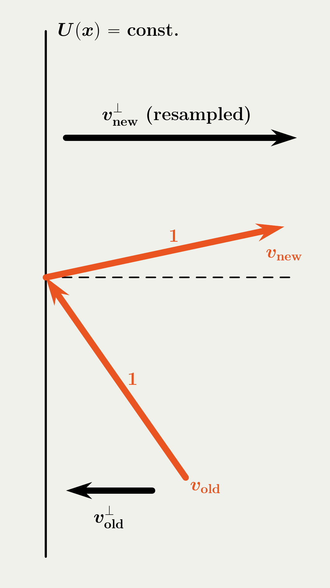
2.2 Jump Mechanisms in BPS vs. FECMC
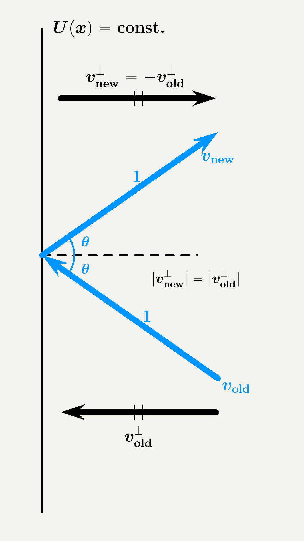
Reflection

\Large +

Refreshment \rho

\Large\fallingdotseq

Stochastic Reflection

2.3 Empirical Comparison: BPS vs. FECMC
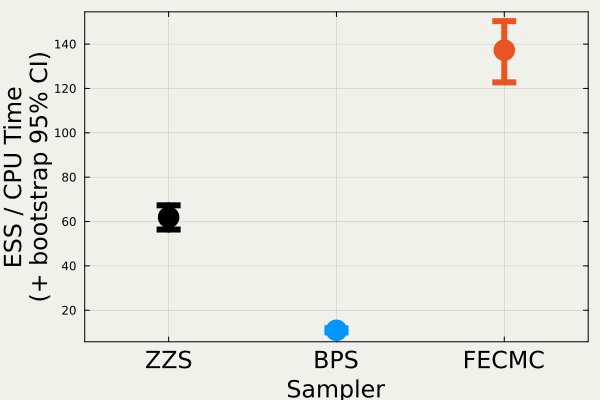
Effective Sample Size of U(x)=\|x\|^2, the negative log-density of 100 dimensional standard Gaussian, estimated over 1000 runs

2.4 Scaling Analysis of MCMCs

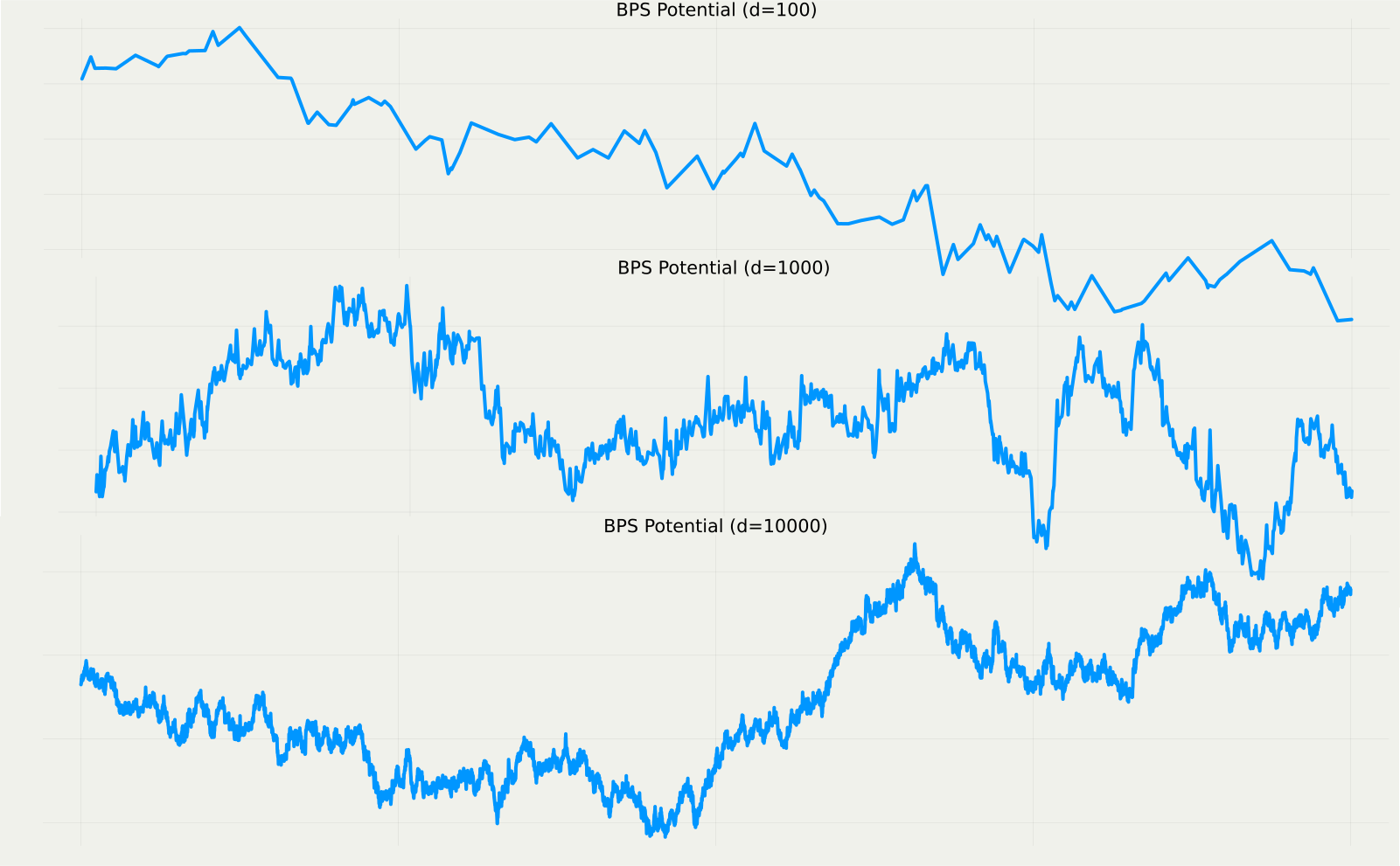
aims to identify the scaling factor \textcolor{#E95420}{d^{\textrm{\,some \,factor}}} that yields a diffusion limit as d\to\infty

\text{Plotting } \textcolor{#0096FF}{Y_t^{(d)}}=\frac{\|\textcolor{#0096FF}{X}_{\textcolor{#E95420}{d}\textcolor{#0096FF}{t}}^{\textcolor{#0096FF}{(d)}}\|^2-d}{\sqrt{d}} \text{ with } d=10^2,10^3,10^4:
2.5 Theorem 1: Diffusion Limits of the Rescaled Energy
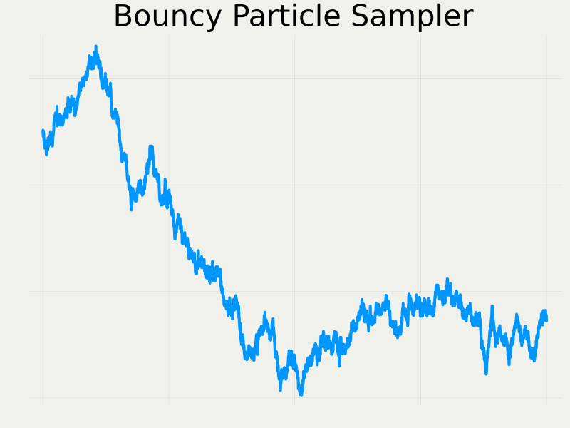
dY_t^{\textcolor{#0096FF}{\text{B}}}=-\frac{\sigma^2_{\textcolor{#0096FF}{\text{B}}}(\rho)}{4}Y_t^{\textcolor{#0096FF}{\text{B}}}\,dt+\sigma_{\textcolor{#0096FF}{\text{B}}}(\rho)\,dB_t \sigma^2_{\textcolor{#0096FF}{\text{B}}}(\rho)=8\int^\infty_0e^{-\rho s}\operatorname{E}[R_0^{\textcolor{#0096FF}{\text{B}}}R_s^{\textcolor{#0096FF}{\text{B}}}]\,ds
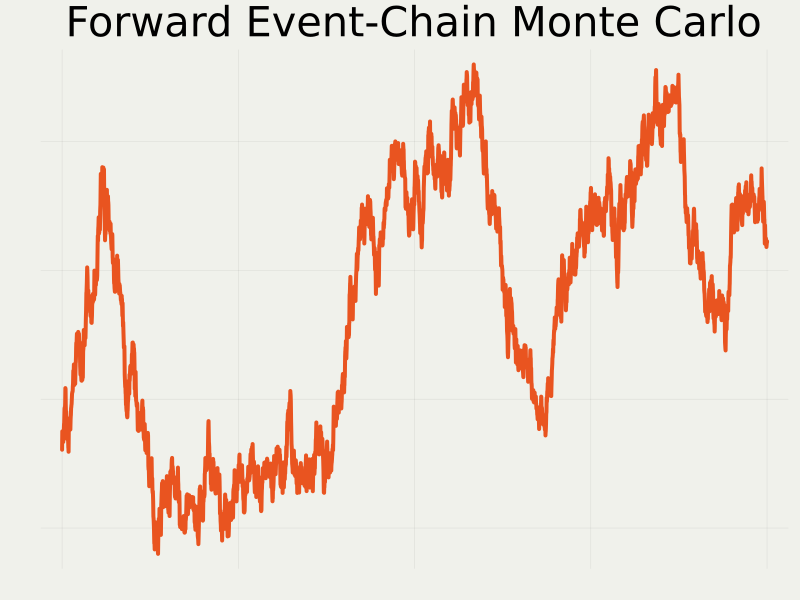
dY_t^{\textcolor{#E95420}{\text{F}}}=-\frac{\sigma^2_{\textcolor{#E95420}{\text{F}}}(\rho)}{4}Y_t^{\textcolor{#E95420}{\text{F}}}\,dt+\sigma_{\textcolor{#E95420}{\text{F}}}(\rho)\,dB_t \sigma^2_{\textcolor{#E95420}{\text{F}}}(\rho)=8\int^\infty_0e^{-\rho s}\operatorname{E}[R_0^{\textcolor{#E95420}{\text{F}}}R_s^{\textcolor{#E95420}{\text{F}}}]\,ds

2.6 Theorem 2: Analytic Expressions of \sigma^2

\begin{align*} \sigma^2_{\textcolor{#E95420}{\text{FECMC}}}(0)&=\sqrt{\frac{32}{\pi}},\\ \sigma^2_{\textcolor{#E95420}{\text{FECMC}}}(\rho)&=\sqrt{\frac{32}{\pi}}\biggr(1-\frac{\left(\rho^2-\rho\sqrt{\frac{\pi}{2}}+\Omega(\rho)\right)^2}{\rho^4\Omega(\rho)(2-\Omega(\rho))}\biggl),\quad\rho>0\\ \sigma^2_{\textcolor{#0096FF}{\text{BPS}}}(\rho)&=\frac{8}{\rho^4}\left(\rho^3-\rho^2\sqrt{\frac{8}{\pi}}+\rho-\sqrt{\frac{8}{\pi}}\frac{\left((1+\rho^2)\Omega(\rho)-\rho^2\right)^2}{\Omega(2\rho)}\right), \end{align*}

where \Omega(\rho)\coloneqq\sqrt{\frac{\pi}{2}}\rho\operatorname{erfcx}\left(\frac{\rho}{\sqrt{2}}\right)=\rho e^{\frac{\rho^2}{2}}\int^\infty_\rho e^{-\frac{t^2}{2}}\,dt is the moment generating function of the standard Rayleigh distribution.

2.7 Theorem 2 (cont.): Plot of \sigma^2
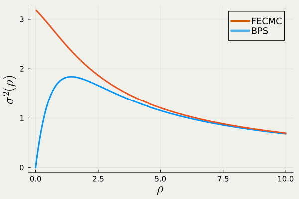
While BPS atteins maximum at non-trivial value of \rho, FECMC achieves maximum at \rho=0

3 Proofs

  • The hypocoercivity / slow-fast structure complicates the standard proof approach
    • The potential U(X_t)=\|X_t\|^2/2 evolves on a slow timescale.
    • Its time derivative R_t:=(X_t|V_t)=dU(X_t)/dt fluctuates on a fast timescale.
  • Spectral properties of R are reflected in \sigma^2

3.1 The Non-Markovianity of the Rescaled Energy Y^d
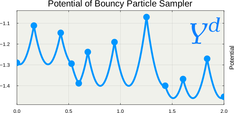
Y^d_{t-} alone cannot determine the speed of Y^d_t at jumps.

3.2 Two Approaches to Non-Markovianity

Augmented Generator (Ethier and Kurtz, 1986)

  • Add enough variables to have a Markovian tuple (Y^d,A^d,B^d,\cdots)

3.3 A Sketch of Proof: A Semimartingale Approach

Doob-Meyer Decomposition (Doléans-Dade and Meyer, 1970)

Y^d is non-Markovian, but is a (special) semimartingale, having Y^d_t=Y^d_0+B^d_t+M^d_t, where B^d is the dual predictable projection of Y^d, and M^d is a local L^2-martingale.

Convergence of Semimartingales (Jacod and Shiryaev, 2003 Theorem IX.3.48)

The convergence of B^d and C^d_t:=\langle M^d\rangle_t (in a suitable sense) to B_t=-\int^t_0\frac{\sigma^2}{4}Y_s\,ds,\quad C_t=\sigma^2t, is part of the sufficient conditions ensuring weak convergence Y^d\Rightarrow Y where dY_t=-\frac{\sigma^2}{4}Y_t\,dt+\sigma\,dB_t.

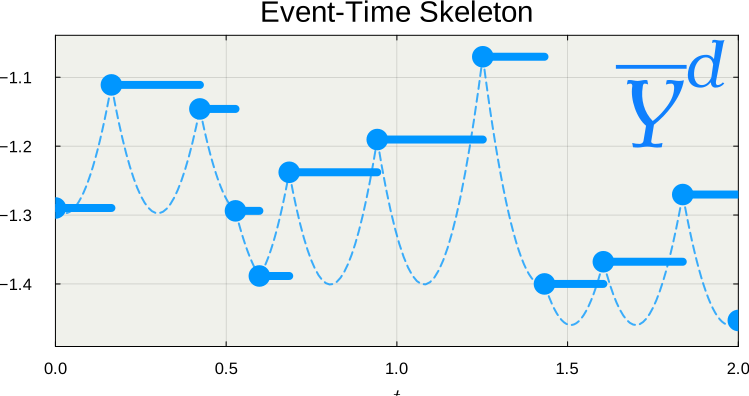
3.4 The Event-Time Skeleton Reveals Local Averaging

Original Potential Process \textcolor{#0096FF}{Y^d}

B^d_t=2\sqrt{d}\int^t_0R^d_{ds-}\,ds,%\quad R_t^d:=\brac{X_t^d,V_t^d}, C^d_t=0.

Difficult to see how C_t=\sigma^2t emerges.
approx.

Event-Time Skeleton \textcolor{#0096FF}{\overline{Y}^d}

\overline{B}^d_t=\sum_{n=1}^{N_t}\operatorname{E}[\Delta\overline{Y}^d_n|\overline{\mathcal{F}}^d_{n-1}] {\tiny \overline{C}^d_t=\sum_{n=1}^{N_t}\left(\operatorname{E}[(\Delta\overline{Y}^d_n)^2|\overline{\mathcal{F}}^d_{n-1}]-\operatorname{E}[\Delta\overline{Y}^d_n|\overline{\mathcal{F}}^d_{n-1}]^2\right).}

Directly connects to the limit.

We then prove the asymptotic equivalence of these two.

3.5 \sigma^2 as the CLT Variance

From Theorem 1, we see \begin{align*} \frac{\sigma^2(\rho)}{4}=2\int^\infty_0e^{-\rho t}\operatorname{E}[R_0R_t]\,dt=\lim_{T\to\infty}\frac{1}{T}\operatorname{Var}\left[\int^T_0R_t\,dt\right]. \end{align*} Therefore, \sigma^2/4 is the asymptotic variance of the ergodic average of R_t.

Pushing the calculation further using Fubini’s theorem, =\operatorname{E}\biggl[R_0\underbrace{\int^\infty_0e^{-\rho t}\operatorname{E}[R_t|R_0]\,dt}_{=:f_\rho(R_0)}\biggr]=\operatorname{E}[R_0f_\rho(R_0)], where f_\rho solves the resolvent equation of R (\rho-\mathcal{L}_R)f_\rho(x)=x where \mathcal{L}_R is the generator of R. This can be explicitly solved. (cf. Bierkens and Lunel, 2022)

3.6 Values of \sigma^2(0) and Poisson equations

Taking \rho\to0, the resolvent equation corresponds to -\mathcal{L}_Rf_0(x)=x.

Sampler Solution \sigma^2(0)=8\mathbb{E}[R_0f_0(R_0)]
BPS \displaystyle f_0^{\textcolor{#2780e3}{B}}(x)=\frac{1-x^2}{2} 0
FECMC \displaystyle f_0^{\textcolor{#E95420}{F}}(x)=\frac14-\frac12\min(x,0)^2 \displaystyle\sqrt{\frac{32}{\pi}}

4 Asymptotic Variance Estimation for PDMP in High Dimensions

There is a stark difference between the ergodic averages

\text{PDMP}\quad\widehat{h}_T^{\textcolor{#E95420}{\text{PDMP}}}=\frac{1}{T}\int^T_0h(\textcolor{#E95420}{X}_{\textcolor{#E95420}{t}}^{\textcolor{#E95420}{(d)}})\,dt,\quad t\in[0,T], \text{classical MCMC}\quad\widehat{h}_N^{\textcolor{#0096FF}{\text{MCMC}}}=\frac{1}{N}\sum_{n=1}^Nh(\textcolor{#0096FF}{X_n^{(d)}}),\quad n=1,\cdots,N.

Estimators for quadratic variation are equivalent to batch means estimators applied to time derivative R.

4.1 Implications of the Diffusion Limit Results

Informal Corollary (Relationship between \sigma^2 and ESS)

The effective sample size (ESS) for estimating U with a trajectory of length \textcolor{#E95420}{d}T is given by \operatorname{ESS}(U)\fallingdotseq\frac{\sigma^2}{8}T\qquad(d\to\infty).

[Proof] The Monte Carlo estimator (= ergodic average of \textcolor{#E95420}{\{X_t\}}) \widehat{h}_T^d:=\frac{1}{T}\int^T_0U(\textcolor{#E95420}{X_t^{(d)}})\,dt has the following variance ratio under a double limit: \lim_{T\to\infty}\lim_{d\to\infty}T\frac{\operatorname{Var}[\widehat{h}_{\textcolor{#E95420}{d}T}^d]}{\operatorname{Var}_\pi[U]}=\frac{8}{\sigma^2}\approx2.50\cdots. ESS equals the inverse of this variance ratio.

4.2 Theory Matches Practice: FECMC vs. BPS
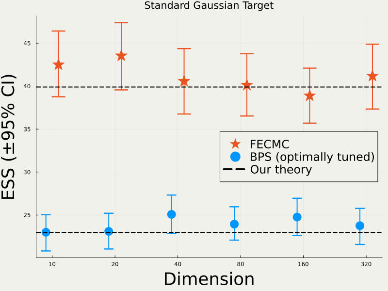
ESS for U estimated over 1000 runs. Every bootstrap CI contains the theoretical limiting value {8}/{\sigma^2}.

4.3 Asymptotic Variance Estimation for MCMC
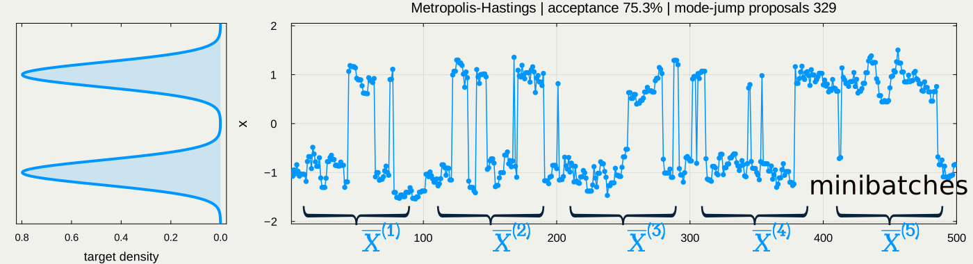
A practical issue: Does this trajectory suffice for mean estimation? → A solution: asymptotic variance estimation

\text{Markov Chain CLT: }\quad\frac{1}{\sqrt{N}}\sum_{n=1}^NX_n\Rightarrow N(0,\sigma^2_{\text{asym}})\quad(N\to\infty). For mini-batches b=1,\cdots,B with length m:=N/B, \operatorname*{{Batch\; Means\; Estimator:}}_{\text{(for mean estimation)}} \text{ }\quad\widehat{\sigma^2}_\text{asym}:=\frac{m}{B-1}\sum_{b=1}^B\left(\textcolor{#0096FF}{\overline{{X}}^{(b)}}-\textcolor{#0096FF}{\overline{{X}}}\right)^2, where \textcolor{#0096FF}{\overline{{X}}^{(b)}}=\frac{1}{m}\sum_{n=1}^m\textcolor{#0096FF}{X_{n+(b-1)m}} is the mean over the b-th batch.

4.4 Optimal Batch Size for Classical MCMC & PDMP
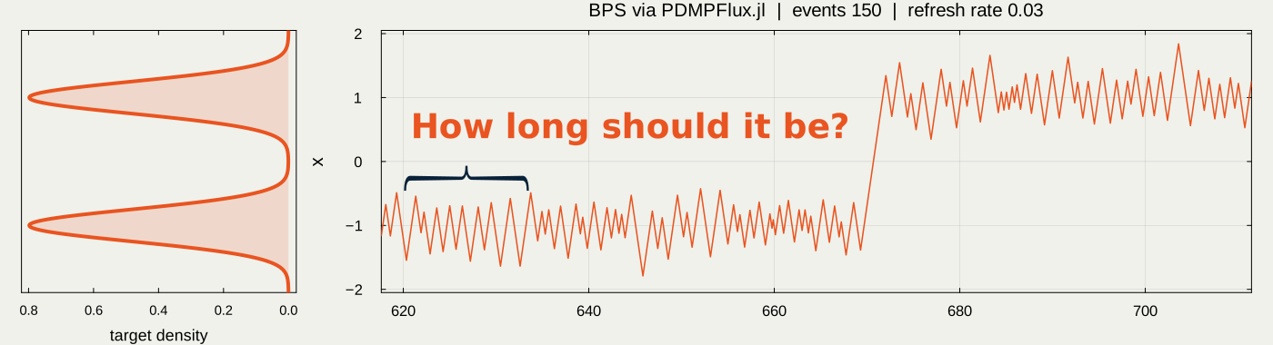
Due to the continuous-time nature, batch size selection becomes a nontrivial problem for PDMPs.

MSE Minimizing Batch Size for Classical MCMC (Liu et al., 2022)

m_{\text{opt}}=\left(\frac{\gamma_{\text{disc}}}{\sigma_{\text{asym}}^2}\right)^{\frac{2}{3}}N^{\frac{1}{3}} minimizes the MSE asymptotically under m\to\infty,\qquad N/m\to\infty, for a sufficiently mixing Markov chain \{\textcolor{#0096FF}{X_n}\}.

Bias Minimizing Batch Size for PDMP (S. & Kamatani 2026+)

Analogously, with \gamma_{\text{disc}}=2\sum_{k=0}^\infty k\operatorname{Cov}[\textcolor{#0096FF}{X_0},\textcolor{#0096FF}{X_k}] replaced by \gamma_{\text{cont}}=2\int^\infty_0t\operatorname{Cov}[\textcolor{#E95420}{X_0},\textcolor{#E95420}{X_t}]\,dt.

4.5 Diffusivity Estimation for High-dimensional PDMPs

= Quadratic Variation (QV) Estimation under Misspecification
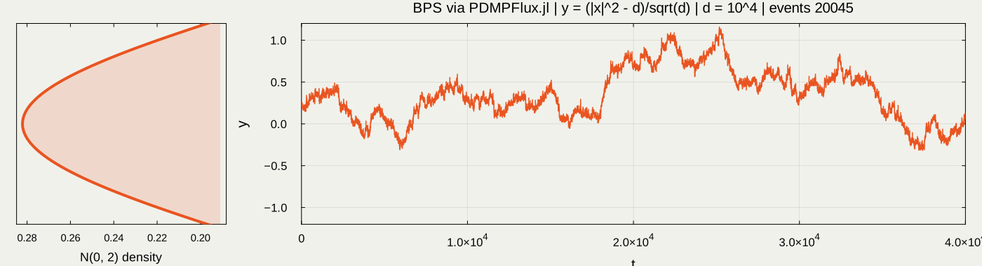
Plot of Y_t^d:=(|\textcolor{#E95420}{X^d}_{d\textcolor{#E95420}{t}}|^2-d)/\sqrt{d} when d=10^4. The trajectory converges to dY_t=-\frac{\sigma^2}{4} Y_t\,dt+\sigma\,dB_t as d\to\infty

The Realized Volatility estimator (Barndorff-Nielsen and Shephard, 2002) \widehat{Q}^d:=\frac{1}{T}\sum_{n=1}^N\biggr(Y_{\Delta n}^d-Y_{\Delta(n-1)}^d\biggl)^2,\quad T=\Delta N, converges to \sigma^2 under the conditions \Delta\to0,\quad d\to\infty,\quad\Delta d\to\infty.

4.6 Experiment: QV Estimator Improves with Dimension
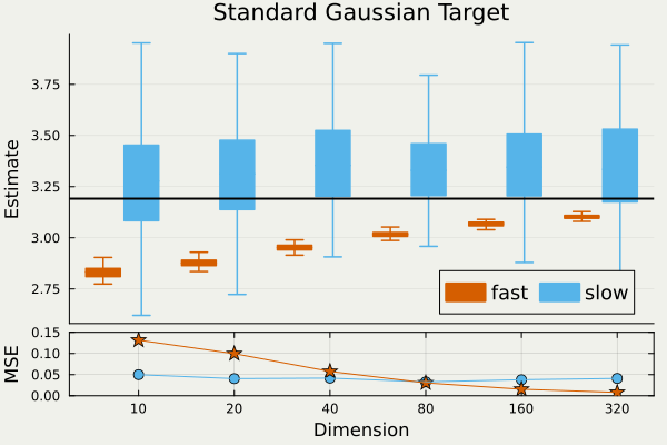
slow corresponds to the Batch Means estimator, fast corresponds to the Realized Variation estimator

4.7 Experiment (cont.): QV Estimator Improvement
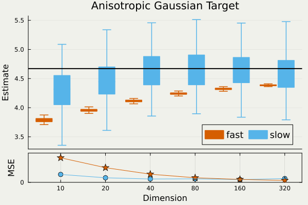
slow corresponds to the Batch Means estimator, fast corresponds to the Realized Variation estimator

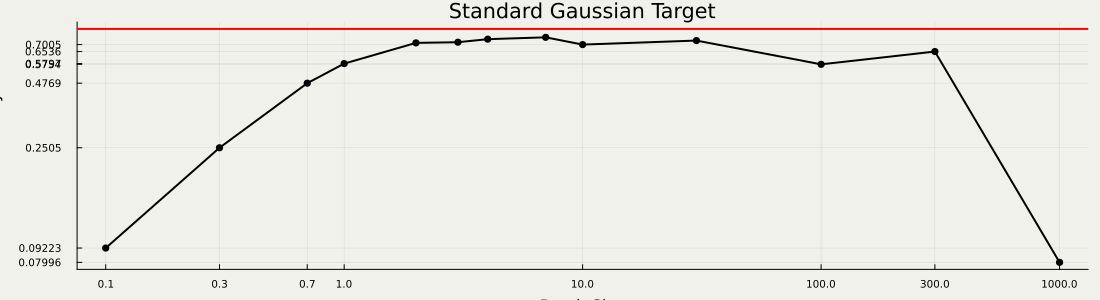
4.8 Batch Size Selection for the QV Estimator

\fallingdotseq selecting the sampling step size \Delta under Misspecification (Aït-Sahalia et al., 2011)
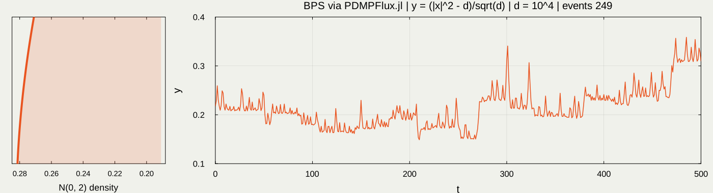
Plot of Y_t^d:=(|\textcolor{#E95420}{X^d}_{d\textcolor{#E95420}{t}}|^2-d)/\sqrt{d} when d=10^4. Taking a closer look, the trajectory is an ODE, a `microstructure noise’

For too small / large \Delta, \widehat{Q}^{d}(\Delta)\approx0. The optimal choice seems to be \Delta=O(d^{1/2}).
Conclusion

  1. Reducing redundant noise produces a more efficient algorithm: BPS → FECMC
    • FECMC has larger \sigma^2 because its reflection is not specular
  2. Continuous-time MCMC allows more efficient estimators for asymptotic variance
    • potentially works whenever a diffusion limit exists
    • with a sensible choice of the batch size

References

Aït-Sahalia, Y., Mykland, P. A., and Zhang, L. (2011). Ultra High Frequency Volatility Estimation with Dependent Microstructure Noise. Journal of Econometrics, 160(1), 160–175.
Barndorff-Nielsen, O. E., and Shephard, N. (2002). Estimating Quadratic Variation using Realized Variance. Journal of Applied Econometrics, 17(5), 457–477.
Bierkens, J., Fearnhead, P., and Roberts, G. (2019). The Zig-Zag Process and Super-Efficient Sampling for Bayesian Analysis of Big Data. The Annals of Statistics, 47(3), 1288–1320.
Bierkens, J., and Lunel, S. M. V. (2022). Spectral analysis of the zigzag process. Annales de l’Institut Henri Poincaré, Probabilités Et Statistiques, 58(2), 827–860.
Bouchard-Côté, A., Vollmer, S. J., and Doucet, A. (2018). The Bouncy Particle Sampler: A Nonreversible Rejection-Free Markov Chain Monte Carlo Method. Journal of the American Statistical Association, 113(522), 855–867.
Cattiaux, P., Chafai, D., and Guillin, A. (2011). Central limit theorems for additive functionals of ergodic markov diffusions processes.
Deligiannidis, G., Paulin, D., Bouchard-Côté, A., and Doucet, A. (2021). Randomized Hamiltonian Monte Carlo as scaling limit of the bouncy particle sampler and dimension-free convergence rates. The Annals of Applied Probability, 31(6), 2612–2662.
Doléans-Dade, C., and Meyer, P.-A. (1970). Intégrales Stochastiques par Rapport aux Martingales Locales. Séminaire de Probabilités, 4, 77–107.
Ethier, S. N., and Kurtz, T. G. (1986). Markov processes: Characterization and convergence. John Wiley & Sons, Inc.
Jacod, J., and Shiryaev, A. N. (2003). Limit Theorems for Stochastic Processes,Vol. 288. Springer Berlin, Heidelberg.
Liu, Y., Vats, D., and Flegal, J. M. (2022). Batch Size Selection for Variance Estimators in MCMC. Methodology and Computing in Applied Probability, 24(1), 65–93.
Michel, M., Durmus, A., and Sénécal, S. (2020). Forward Event-Chain Monte Carlo: Fast Sampling by Randomness Control in Irreversible Markov Chains. Journal of Computational and Graphical Statistics, 29(4), 689–702.