
最適輸送とは何か?
歴史と概観
2024-09-03
Python で最適輸送写像を計算する方法を解説する. 直接最適輸送問題を POT (Python Optimal Transport) で解く.この方法は原子の数 \(N\) に対して \(O(N^3\log N)\) の複雑性を持つ. 一方で,エントロピー正則化項 \(\epsilon\operatorname{Ent}(\pi)\) を導入したエントロピー最適輸送問題は Sinkhorn アルゴリズムで高速に解くことができる. これには OTT-JAX パッケージを用いる. \(\epsilon\to0\) の極限で元の最適輸送問題の解を得る.
A Blog Entry on Bayesian Computation by an Applied Mathematician
$$
$$
def plot_weighted_points(
    ax,
    x, a,
    y, b,
    title=None, x_label=None, y_label=None
):
  ax.scatter(x[:,0], x[:,1], s=5000*a, c='r', edgecolors='k', label=x_label)
  ax.scatter(y[:,0], y[:,1], s=5000*b, c='b', edgecolors='k', label=y_label)
  for i in range(np.shape(x)[0]):
      ax.annotate(str(i+1), (x[i,0], x[i,1]),fontsize=30,color='black')
  for i in range(np.shape(y)[0]):
      ax.annotate(str(i+1), (y[i,0], y[i,1]),fontsize=30,color='black')
  if x_label is not None or y_label is not None:
    ax.legend(fontsize=20)
  ax.axis('off')
  ax.set_title(title, fontsize=25)

def plot_assignement(
    ax,
    x, a,
    y, b,
    optimal_plan,
    title=None, x_label=None, y_label=None
):
  plot_weighted_points(
    ax=ax,
    x=x, a=a,
    y=y, b=b,
    title=None,
    x_label=x_label, y_label=y_label
  )
  for i in range(optimal_plan.shape[0]):
      for j in range(optimal_plan.shape[1]):
          ax.plot([x[i,0], y[j,0]], [x[i,1], y[j,1]], c='k', lw=30*optimal_plan[i,j], alpha=0.8)
  ax.axis('off')
  ax.set_title(title, fontsize=30)

def plot_assignement_1D(
    ax,
    x, y,
    title=None
):
  plot_points_1D(
    ax,
    x, y,
    title=None
  )
  x_sorted = np.sort(x)
  y_sorted = np.sort(y)
  assert len(x) == len(y), "x and y must have the same shape."
  for i in range(len(x)):
    ax.hlines(
        y=0,
        xmin=min(x_sorted[i], y_sorted[i]),
        xmax=max(x_sorted[i], y_sorted[i]),
        color='k',
        lw=10
    )
  ax.axis('off')
  ax.set_title(title, fontsize=30)

def plot_points_1D(
    ax,
    x, y,
    title=None
):
  n = len(x)
  a = np.ones(n) / n
  ax.scatter(x, np.zeros(n), s=1000*a, c='r')
  ax.scatter(y, np.zeros(n), s=1000*b, c='b')
  min_val = min(np.min(x), np.min(y))
  max_val = max(np.max(x), np.max(y))
  for i in range(n):
      ax.annotate(str(i+1), xy=(x[i], 0.005), size=30, color='r', ha='center')
  for j in range(n):
      ax.annotate(str(j+1), xy=(y[j], 0.005), size=30, color='b', ha='center')
  ax.axis('off')
  ax.plot(np.linspace(min_val, max_val, 10), np.zeros(10))
  ax.set_title(title, fontsize=30)

def plot_consistency(
    ax,
    reg_strengths,
    plan_diff, distance_diff
):
  ax[0].loglog(reg_strengths, plan_diff, lw=4)
  ax[0].set_ylabel('$||P^* - P_\epsilon^*||_F$', fontsize=25)
  ax[1].tick_params(which='both', size=20)
  ax[0].grid(ls='--')
  ax[1].loglog(reg_strengths, distance_diff, lw=4)
  ax[1].set_xlabel('Regularization Strength $\epsilon$', fontsize=25)
  ax[1].set_ylabel(r'$ 100 \cdot \frac{\langle C, P^*_\epsilon \rangle - \langle C, P^* \rangle}{\langle C, P^* \rangle} $', fontsize=25)
  ax[1].tick_params(which='both', size=20)
ax[1].grid(ls='--')pip install POT
pip install cloudpickleimport ot
import numpy as np
import os
from typing import Callable
import matplotlib.pyplot as pltWe will solve the Bakeries/Cafés problem of transporting croissants from a number of Bakeries to Cafés.
We use fictional positions, production and sale numbers. We impose that the total croissant production is equal to the number of croissants sold, so that Bakeries and Cafés can be represented as measures with the same total mass. Then, up to normalization, they can be processed as probability measures.
Mathematically, we have acess to the position of the \(m\) Bakeries as points in \(\mathbb{R}^2\) via \(x \in \mathbb{R}^{n \times 2}\) and their respective production via \(a \in \mathbb{R}^m\) which describe the source point cloud. The Cafés where the croissants are sold are also defined by their position \(y \in \mathbb{R}^{m \times 2}\) and the quantity of croissants sold by \(b \in \mathbb{R}^{m}\).
Afterwards, the Bakeries are represented by the probability measure \(\mu = \sum_{i=1}^n a_i \delta_{x_i}\) and the Cafés by \(\nu = \sum_{j=1}^n b_j \delta_{y_j}\). Calculating the optimal assignment of the croissants delivered by the Bakeries to the Cafés remains to calculating the optimal transport between the probability measures \(\mu\) and \(\nu\).
Let’s download the data and check that the total croissant production is equal to the number of croissants sold.
# Load the data
import pickle
from urllib.request import urlopen
import cloudpickle as cp

croissants = cp.load(urlopen('https://marcocuturi.net/data/croissants.pickle'))

bakery_pos = croissants['bakery_pos']
bakery_prod = croissants['bakery_prod']
cafe_pos = croissants['cafe_pos']
cafe_prod = croissants['cafe_prod']

print('Bakery productions =', bakery_prod)
print('Total number of croissants =', bakery_prod.sum())
print("")
print('Café sales =', cafe_prod)
print('Total number of croissants sold =', cafe_prod.sum())
Bakery productions = [31. 48. 82. 30. 40. 48. 89. 73.]
Total number of croissants = 441.0
Café sales = [82. 88. 92. 88. 91.]
Total number of croissants sold = 441.0We now normalize the weight vectors \(a\) and \(b\), i.e. the production and the sales, to deal with probability measures.
bakery_prod = bakery_prod / bakery_prod.sum()
cafe_prod = cafe_prod / cafe_prod.sum()
Then, we plot the probability measures (the weighted point clouds) in \(\mathbb{R}^2\).
fig, ax = plt.subplots(figsize=(10, 8))
plot_weighted_points(
    ax,
    x=bakery_pos,
    a=bakery_prod,
    x_label="Bakeries",
    y=cafe_pos,
    y_label="Cafés",
    b=cafe_prod,
    title="Bakeries and Cafés"
)
plt.show()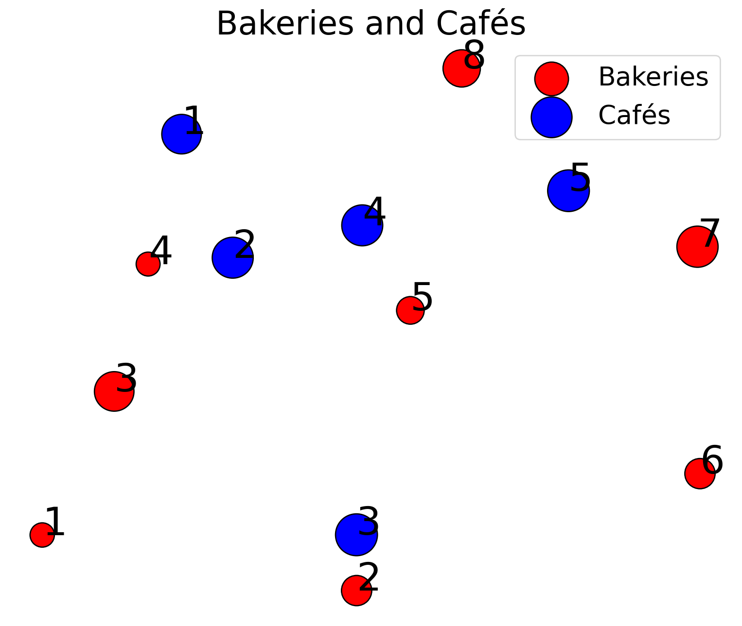
To compute the optimal transport, we will consider three different costs:
Note that we expect different optimal transport plans for different costs.
Question:
Answer:
bakery_posarray([[184.86464733, 201.8163543 ],
[449.3486663 , 168.40784664],
[245.41756746, 288.12166576],
[273.95400109, 364.68282915],
[494.58935376, 336.8424061 ],
[738.19305545, 238.70491485],
[736.10502372, 375.12298779],
[537.74200949, 482.30861653]])cafe_posarray([[302.08410452, 442.78633642],
[345.1162221 , 368.52123027],
[449.226184 , 201.94529124],
[454.08464888, 387.95508982],
[627.60125204, 408.7770822 ]])def get_cost_matrix(
x: np.ndarray,
y: np.ndarray,
cost_fn: Callable
) -> np.ndarray:
"""
Compute the pairwise cost matrix between the n points in ``x`` and the m points in ``y``.
It should output a matrix of size n x m.
"""
return np.array([cost_fn(x_,y_) for x_ in x for y_ in y]).reshape(x.shape[0],y.shape[0])
# compute cost matrices for different costs
C_l1 = get_cost_matrix(
x=bakery_pos, y=cafe_pos,
cost_fn= lambda x,y : sum(np.abs(x-y))
)
C_l2 = get_cost_matrix(
x=bakery_pos, y=cafe_pos,
cost_fn= lambda x,y : sum((x-y)**2)
)
C_l2_sq = get_cost_matrix(
x=bakery_pos, y=cafe_pos,
cost_fn= lambda x,y : sum(np.sqrt((x-y)**2))
)
# print shapes of cost matrices
print(
f"Shape of C_l1: {C_l1.shape}\n"
f"Shape of C_l2: {C_l2.shape}\n"
f"Shape of C_l2_sq: {C_l2_sq.shape}"
)Shape of C_l1: (8, 5)
Shape of C_l2: (8, 5)
Shape of C_l2_sq: (8, 5)We can now compute the Optimal Transport plan to transport the croissants from the bakeries to the cafés, for the three different costs.
Question:
ot.emd function. It has an option to display the results.Remark: See https://pythonot.github.io/ for informations on the ot.emd function.
Answer:
def compute_transport(
    C: np.ndarray,
    a: np.ndarray,
    b: np.ndarray,
    verbose: bool = False,
):
  """
  Compute the optimal transport plan and the optimal transport cost
  for cost matrix ``C`` and weight vectors $a$ and $b$.
  If ``verbose`` is set to True, it displays the results.
  """
  optimal_plan = ot.emd(a,b,C)
  optimal_cost = np.sum(optimal_plan * C)
  if verbose:
    print(
        f"optimal transport plan: \n{optimal_plan}"
    )
    print(
        f"transport cost: {optimal_cost}"
    )
  return optimal_plan, optimal_cost
# l1 geometry
print("l1 geometry:")
optimal_plan_l1_croissant, optimal_cost_l1_croissant = compute_transport(
C=C_l1,
a=bakery_prod,
b=cafe_prod,
verbose=True
)l1 geometry:
optimal transport plan:
[[0.07029478 0. 0. 0. 0. ]
[0. 0. 0.10884354 0. 0. ]
[0.05442177 0.13151927 0. 0. 0. ]
[0. 0.06802721 0. 0. 0. ]
[0. 0. 0. 0.09070295 0. ]
[0. 0. 0.09977324 0.00453515 0.00453515]
[0. 0. 0. 0. 0.20181406]
[0.06122449 0. 0. 0.10430839 0. ]]
transport cost: 177.28420815406028# l2 geometry
print("l2 geometry:")
optimal_plan_l2_croissant, optimal_cost_l2_croissant = compute_transport(
C=C_l2,
a=bakery_prod,
b=cafe_prod,
verbose=True
)l2 geometry:
optimal transport plan:
[[0. 0.07029478 0. 0. 0. ]
[0. 0. 0.10884354 0. 0. ]
[0.11791383 0.06802721 0. 0. 0. ]
[0.06802721 0. 0. 0. 0. ]
[0. 0.06122449 0. 0.02947846 0. ]
[0. 0. 0.09977324 0.00453515 0.00453515]
[0. 0. 0. 0. 0.20181406]
[0. 0. 0. 0.16553288 0. ]]
transport cost: 24576.370543882178# squared l2 geometry
print("squared l2 geometry:")
optimal_plan_l2_sq_croissant, optimal_cost_l2_sq_croissant = compute_transport(
C=C_l2_sq,
a=bakery_prod,
b=cafe_prod,
verbose=True
)squared l2 geometry:
optimal transport plan:
[[0.07029478 0. 0. 0. 0. ]
[0. 0. 0.10884354 0. 0. ]
[0.05442177 0.13151927 0. 0. 0. ]
[0. 0.06802721 0. 0. 0. ]
[0. 0. 0. 0.09070295 0. ]
[0. 0. 0.09977324 0.00453515 0.00453515]
[0. 0. 0. 0. 0.20181406]
[0.06122449 0. 0. 0.10430839 0. ]]
transport cost: 177.28420815406028Now, we can visualize the assignement induced by each geometry.
fig, ax = plt.subplots(
    1, 3, figsize=(9*3, 7)
)
plans = [optimal_plan_l1_croissant,
         optimal_plan_l2_croissant,
         optimal_plan_l2_sq_croissant]
titles = [r"$\ell_1$ geometry", r"$\ell_2$ geometry", r"$\ell_2^2$ geometry"]

for axes, plan, title in zip(ax, plans, titles):
  plot_assignement(
      ax=axes,
      x=bakery_pos, a=bakery_prod, x_label="Bakeries",
      y=cafe_pos, b=cafe_prod, y_label="Cafés",
      optimal_plan=plan,
      title=title
  )
plt.show()
Let assume in this subsection that the cost is of the form \(c(x, y) = \|x - y\|_p^q\) with \(p, q \geq 1\), which covers the costs we considered in the previous examples, and that the points are in \(\mathbb{R}\), i.e. \(x_1, ..., x_n, y_1, ... , y_n \in \mathbb{R}\). Then, computing OT boils down to sorting the points. Indeed, for all costs of the above form, the optimal permutation between \(x\) and \(y\) is \(\sigma^* = \sigma_x^{-1} \circ \sigma_y\) where \(\sigma_x\) is the permutation sorting the \(x_i\) and \(\sigma_y\) the one sorting the \(y_i\). In particular, one has:
\[ W_c(\mu, \nu) = \frac{1}{n} \sum_{i=1}^n c(x_i, y_{\sigma_x^{-1} \circ \sigma_y(i)}) = \frac{1}{n} \sum_{i=1}^n c(x_{\sigma_x(i)}, y_{\sigma_y(i)}) \]
Thus, to compute the optimal transport cost, it is sufficient to sort \(x\) and \(y\).
Let’s check this fact on an example, by comparing the transport cost obtained by sorting the points to the one obtained with the function ot.emd. To simplify, we generate points \(x,y \subset \mathbb{R}\) s.t. \(x\) is sorted, i.e. \(\sigma_x = I_d\) and then \(\sigma^*=\sigma_y\). Therefore, computing the optimal assignement amounts to sort \(y\).
# generate points
n = 5
x = np.arange(0, 2*n, 2) + .25 * np.random.normal(size=(n,))
a = np.ones(n) / n
y = np.arange(1, 2*n+1, 2) + .25 * np.random.normal(size=(n,))
np.random.shuffle(y)
b = np.ones(n) / n

# plot points
fig, ax = plt.subplots(figsize=(12, 6))
plot_points_1D(
    ax,
    x, y,
    title="1D points"
)
Question:
ot.emd.Answer:
# sort the points
y_sorted = np.sort(y)

# get optimal assignment as a vector
assignment = np.argsort(y)

# transform it to a transport plan
optimal_plan = np.zeros((n,n))
for i, idx in enumerate(assignment):
    optimal_plan[i, idx] = 1 / n
print(
    f"optimal transport plan obtained by sorting the points:\n {optimal_plan}"
)

# The result doesn't match the lecturer's
optimal transport plan obtained by sorting the points:
[[0. 0. 0. 0.2 0. ]
[0.2 0. 0. 0. 0. ]
[0. 0. 0. 0. 0.2]
[0. 0.2 0. 0. 0. ]
[0. 0. 0.2 0. 0. ]]# l1 geometry
print("l1 geometry:")
C_l1 = get_cost_matrix(
x=x, y=y,
cost_fn=lambda x,y: np.sum(np.abs(x - y))
)
optimal_plan_l1, optimal_cost_l1 = compute_transport(
C=C_l1,
a=a,
b=b,
verbose=True
)
print(
f"is it equal to the one obtained by sorting the points? "
f"{np.array_equal(optimal_plan_l1, optimal_plan)}"
)l1 geometry:
optimal transport plan:
[[0. 0. 0. 0.2 0. ]
[0.2 0. 0. 0. 0. ]
[0. 0. 0. 0. 0.2]
[0. 0.2 0. 0. 0. ]
[0. 0. 0.2 0. 0. ]]
transport cost: 1.149278108705205
is it equal to the one obtained by sorting the points? True# squared l2 geometry
def is_permutation(matrix):
"""
Check if a given matrix is a permutation matrix.
"""
n, m = matrix.shape
if n != m:
return False
row_sum = np.sum(matrix, axis=1)
col_sum = np.sum(matrix, axis=0)
return np.all(row_sum == 1) and np.all(col_sum == 1) and np.all((matrix == 0) | (matrix == 1))
C_l2_sq = get_cost_matrix(
x=x, y=y,
cost_fn=lambda x,y: np.sum((x - y) ** 2)
)
optimal_plan_l2_sq, optimal_cost_l2_sq = compute_transport(
C=C_l2_sq,
a=a,
b=b,
verbose=True
)
print(
f"is permutation matrix? {is_permutation(optimal_plan_l2_sq)}"
)
print(
f"is it equal to the one obtained by sorting the points? "
f"{np.array_equal(optimal_plan_l2_sq, optimal_plan)}"
)optimal transport plan:
[[0. 0. 0. 0.2 0. ]
[0.2 0. 0. 0. 0. ]
[0. 0. 0. 0. 0.2]
[0. 0.2 0. 0. 0. ]
[0. 0. 0.2 0. 0. ]]
transport cost: 1.3651629169059696
is permutation matrix? False
is it equal to the one obtained by sorting the points? TrueFinally, one can plot the assignement.
fig, ax = plt.subplots(figsize=(12, 6))
plot_assignement_1D(
    ax,
    x, y,
    title="1D assignement"
)
plt.show()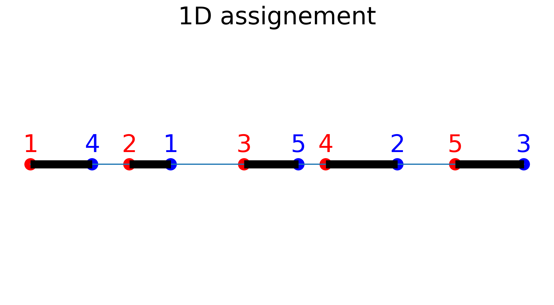
In real ML applications, we often deal with large numbers of points. In this case, cubic complexity linear programming algorithms are too costly. This motivates (among other reasons) the regularized approach \[ \min_{P \in \mathcal{U}(a,b)} \langle C, P \rangle + \epsilon \sum_{ij} P_{ij} [ \log(P_{ij}) - 1]. \] For \(\epsilon\) is sufficiently small, one expects to recover an approximation of the original optimal transport plan.
In order to solve this problem, one can remark that the optimality conditions imply that a solution \(P_\epsilon^*\) necessarily is of the form \(P_\epsilon^* = \text{diag}(u) \, K \, \text{diag}(v)\), where \(K = \exp(-C/\epsilon)\) and \(u,v\) are two non-negative vectors.
\(P_\epsilon^*\) should verify the constraints, i.e. \(P_\epsilon^* \in U(a,b)\), so that \[ P_\epsilon^* 1_m = a \text{ and } (P_\epsilon^*)^T 1_n = b \] which can be rewritten as \[ u \odot (Kv) = a \text{ and } v \odot (K^T u) = b \]
Then Sinkhorn’s algorithm alternates between the resolution of these two equations, and reads at iteration \(t\): \[ u^{t+1} \leftarrow \frac{a}{Kv^t} \text{ and } v^{t+1} \leftarrow \frac{b}{K^T u^{t+1}} \]
Usually, it starts from \(v^{0} = \mathrm{1}_m\) and alternate the above updates until \(\|u^{t+1} \odot (Kv^{t+1}) - a\|_1 + \|v^{t+1} \odot (K^T u^{t+1}) - b\|_1 \leq \tau\), where \(\tau > 0\) is a fixed convergence threshold. Actually, since at the end of each iteration, one exactly has \(v^{t+1} \odot (K^T u^{t+1}) = b\), it just remains to test if \(\|u^{t+1} \odot (Kv^{t+1}) - a\|_1 \leq \tau\).
From an entropic optimal transport plan \(P^*_\epsilon\), we can approximate the optimal transport cost by \(\sum_{i,j=1}^n P^*_{\epsilon_{ij}} C_{ij} = ⟨C, P^*_\epsilon⟩\). For the rest of the section, we call this quantity the entropic optimal transport cost.
In this section, you will implement your own version of the Sinkhorn Algorithm.
Question: Complete the following Sinkhorn algorithm, by:
Remark: you should also use also a maximum number of iterations max_iter, to stop the algorithm after a fixed number of iterations if the convergence is not reached.
Answer:
def sinkhorn(
    a: np.ndarray,
    b: np.ndarray,
    C: np.ndarray,
    epsilon: float,
    max_iters: int = 100,
    tau: float = 1e-4
) -> np.ndarray:
    """
    Sinnkhorn's algorithm. It should output the optimal transport plan.
    """

    K = np.exp( -C / epsilon )
    n, m = a.shape[0], b.shape[0]
    v = np.ones((m,))
    for _ in range(max_iters):
        u = a / K.dot(v)
        v = b / K.transpose().dot(u)
    return u[:,None] * v[None,:] * K  # u_i, v_j, K_ij
P = sinkhorn(a, b, C_l2_sq, epsilon=1)
print(P.sum(axis=0))
print(P.sum(axis=1))[0.2 0.2 0.2 0.2 0.2]
[0.19757988 0.19787653 0.20030352 0.20090692 0.20333316]P = sinkhorn(a, b, C_l2_sq, epsilon=1, max_iters=1000)
print(P.sum(axis=0))
print(P.sum(axis=1))[0.2 0.2 0.2 0.2 0.2]
[0.19997544 0.1999764 0.20000093 0.20000297 0.20004426]def sinkhorn(
a: np.ndarray,
b: np.ndarray,
C: np.ndarray,
epsilon: float,
max_iters: int = 100,
tau: float = 1e-4
) -> np.ndarray:
"""
Sinnkhorn's algorithm. It should output the optimal transport plan.
"""
K = np.exp( -C / epsilon )
n, m = a.shape[0], b.shape[0]
v = np.ones((m,))
for i in range(max_iters):
u = a / K.dot(v)
v = b / K.transpose().dot(u)
if i % 10 == 0:
# compute row sum D(u) K D(v) = u * Kv
if np.sum(np.abs(u * K.dot(v) - a)) < tau:
print('early termination: ' + str(i))
break
return u[:,None] * v[None,:] * K # u_i, v_j, K_ijP = sinkhorn(a, b, C_l2_sq, epsilon=1, max_iters=1000)
print(P.sum(axis=0))
print(P.sum(axis=1))early termination: 990
[0.2 0.2 0.2 0.2 0.2]
[0.19997453 0.19997552 0.20000097 0.20000309 0.20004589]P = sinkhorn(a, b, C_l2_sq, epsilon=0.1, max_iters=10000)
print(P.sum(axis=0))
print(P.sum(axis=1))[0.2 0.2 0.2 0.2 0.2]
[0.19995991 0.19997995 0.2 0.20002005 0.2000401 ]Now, we can test the Sinkhorn algorithm on the “croissant” transport example.
Question: * Complete the following fuction that takes as input the cost matrix \(C\) and the weights vectors \(a\) and \(b\) and outputs the entropic optimal transport plan and the entropic optimal transport cost using the sinkhorn function. As for the exact transport, it has an option to display the results. * Use that function on the croissant transport to compute and display the optimal plan and the optimal cost for the \(\ell_1, \ell_2\) and \(\ell_2^2\) geometries. * Each time you run the Sinkhorn algorithm, you should use \(\epsilon = 0.1 \cdot \bar{C}\), with \(\bar{C} = \frac{1}{nm} \sum_{i=1}^n \sum_{j=1}^m C_{ij}\) is the mean of the cost matrix. It remains to adapt the \(\epsilon\) value according to the cost matrix, to control the magnitude of the entries of \(C / \epsilon\). Why this strategy? What will happen if \(\epsilon\) is too small compared to the entries of \(C\)?
Answer:
def compute_transport_sinkhorn(
    C: np.ndarray,
    a: np.ndarray,
    b: np.ndarray,
    epsilon: float,
    max_iters: int = 10_000,
    tau: float = 1e-4,
    verbose: bool = False,
):
  """
  Compute the entropic optimal transport plan and the entropic optimal transport cost
  for cost matrix ``C`` and weight vectors $a$ and $b$.
  If ``verbose`` is set to True, it displays the results.
  """
  optimal_plan_sinkhorn = sinkhorn(a, b, C, epsilon, max_iters, tau)
  optimal_cost_sinkhorn = np.sum(optimal_plan_sinkhorn * C)
  if verbose:
    print(
        f"entropic optimal transport plan: \n{optimal_plan_sinkhorn}"
    )
    print(
        f"entropic transport cost: {optimal_cost_sinkhorn}"
    )
  return optimal_plan_sinkhorn, optimal_cost_sinkhorn
# l1 geometry
print("l1 geometry:")
C_l1 = get_cost_matrix(
x=bakery_pos, y=cafe_pos,
cost_fn=lambda x,y: np.sum(np.abs(x - y))
)
epsilon = 1
optimal_plan_sinkhorn_l1_croissant, optimal_cost_sinkhorn_l1_croissant = compute_transport_sinkhorn(
C=C_l1,
a=bakery_prod,
b=cafe_prod,
epsilon=epsilon,
verbose=True,
)l1 geometry:
early termination: 5970
entropic optimal transport plan:
[[2.70428936e-002 4.32583290e-002 1.34214268e-047 1.83509051e-086
1.62880160e-235]
[3.42773260e-084 1.30691077e-046 1.08827539e-001 1.90100995e-040
1.68731081e-189]
[7.15328153e-002 1.14425257e-001 4.99347632e-122 4.85411038e-086
4.30844293e-235]
[2.61705422e-002 4.18628990e-002 5.77469196e-189 1.77589404e-086
1.57625961e-235]
[1.25908361e-049 4.80057848e-012 2.70172554e-084 9.07098043e-002
1.22406524e-115]
[2.66904088e-052 1.01764013e-014 9.97892408e-002 1.92289196e-004
8.84651301e-003]
[5.95876320e-051 4.18968529e-019 7.18872709e-119 4.29294956e-003
1.97502693e-001]
[6.11947921e-002 7.27950530e-029 1.24902883e-128 1.04351442e-001
5.20381800e-060]]
entropic transport cost: 177.27648952346257plt.imshow(optimal_plan_sinkhorn_l1_croissant)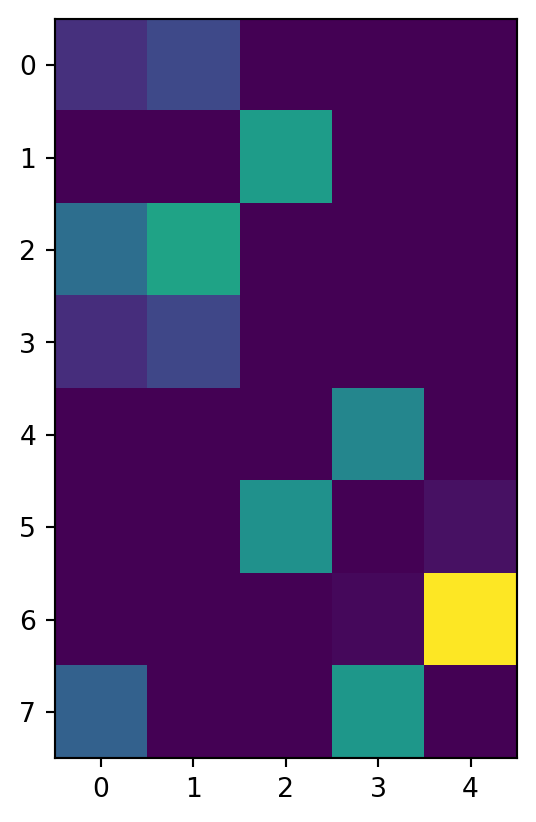
# l2 geometry
print("l2 geometry:")
C_l2 = get_cost_matrix(
    x=bakery_pos, y=cafe_pos,
    cost_fn=lambda x,y: np.linalg.norm(x - y, ord=2)
)
epsilon = np.mean(C_l2_sq) * 0.05 # compute the optimal value to avoid underflow
optimal_plan_sinkhorn_l2_croissant, optimal_cost_sinkhorn_l2_croissant = compute_transport_sinkhorn(
    C=C_l2,
    a=bakery_prod,
    b=cafe_prod,
    epsilon=epsilon,
    verbose=True
)
l2 geometry:
early termination: 6480
entropic optimal transport plan:
[[1.47195199e-002 5.55812693e-002 2.07887308e-066 1.89085801e-083
4.08212986e-215]
[4.71170808e-067 2.26166564e-043 1.08836263e-001 9.74649907e-077
7.01848099e-170]
[4.19924977e-002 1.43964413e-001 2.66725594e-094 2.03490446e-086
7.16649420e-222]
[6.80327467e-002 4.36749516e-013 5.13671791e-141 2.72754187e-101
3.05721358e-239]
[1.24385751e-021 8.02928239e-007 1.04149196e-050 9.07085294e-002
6.66796031e-098]
[8.63129441e-026 1.06829448e-010 9.97805175e-002 4.48903087e-003
4.56691630e-003]
[2.65261029e-046 2.59222291e-040 8.94588488e-063 2.71496095e-025
2.01782290e-001]
[6.11962788e-002 1.70632530e-011 1.98854584e-093 1.04348925e-001
1.28895438e-052]]
entropic transport cost: 139.5030886918118# squared l2 geometry
print("squared l2 geometry:")
C_l2_sq = get_cost_matrix(
x=bakery_pos, y=cafe_pos,
cost_fn=lambda x,y: np.sum((x - y) ** 2)
)
epsilon = np.mean(C_l2_sq) * 0.05 # compute the optimal value to avoid underflow
optimal_plan_sinkhorn_l2_sq_croissant, optimal_cost_sinkhorn_l2_sq_croissant = compute_transport_sinkhorn(
C=C_l2_sq,
a=bakery_prod,
b=cafe_prod,
epsilon=epsilon,
verbose=True
)squared l2 geometry:
early termination: 390
entropic optimal transport plan:
[[9.15185856e-03 6.11459020e-02 2.53416007e-06 9.36830019e-11
5.88710931e-33]
[1.98312263e-09 2.86298466e-05 1.08801507e-01 2.62245737e-07
1.22762517e-18]
[1.02592189e-01 8.33635462e-02 3.95058637e-08 1.25018168e-08
7.16059834e-28]
[6.36539082e-02 4.37874407e-03 9.20213996e-12 8.38044497e-09
1.80226054e-26]
[1.15178824e-03 4.78786088e-02 4.40333811e-04 4.12385828e-02
1.04144097e-10]
[1.27912352e-15 1.00116432e-09 9.93719135e-02 7.28353201e-04
8.73056135e-03]
[5.51097456e-13 1.50024181e-09 4.51186568e-07 4.17827621e-03
1.97618514e-01]
[9.39129734e-03 2.75105187e-03 4.51869851e-10 1.53400990e-01
1.31200779e-07]]
entropic transport cost: 24883.330683517215Now we can display the transportation plans obtained with Sinkhorn’s algortihm, as we did for the exact OT.
fig, ax = plt.subplots(
    1, 3, figsize=(9*3, 7)
)
plans = [optimal_plan_sinkhorn_l1_croissant,
         optimal_plan_sinkhorn_l2_croissant,
         optimal_plan_sinkhorn_l2_sq_croissant]

titles = [r"$\ell_1$ geometry", r"$\ell_2$ geometry", r"$\ell_2^2$ geometry"]

for axes, plan, title in zip(ax, plans, titles):
  plot_assignement(
      ax=axes,
      x=bakery_pos, a=bakery_prod, x_label="Bakeries",
      y=cafe_pos, b=cafe_prod, y_label="Cafés",
      optimal_plan=plan,
      title=title
  )
plt.show()
Note: There always is some transport at every edge in Sinkhorn algorithm’s output.
fig, ax = plt.subplots(
    1, 3, figsize=(9*3, 7)
)
plans = [optimal_plan_l1_croissant,
         optimal_plan_l2_croissant,
         optimal_plan_l2_sq_croissant]

titles = [r"$\ell_1$ geometry", r"$\ell_2$ geometry", r"$\ell_2^2$ geometry"]

for axes, plan, title in zip(ax, plans, titles):
  plot_assignement(
      ax=axes,
      x=bakery_pos, a=bakery_prod, x_label="Bakeries",
      y=cafe_pos, b=cafe_prod, y_label="Cafés",
      optimal_plan=plan,
      title=title
  )
plt.show()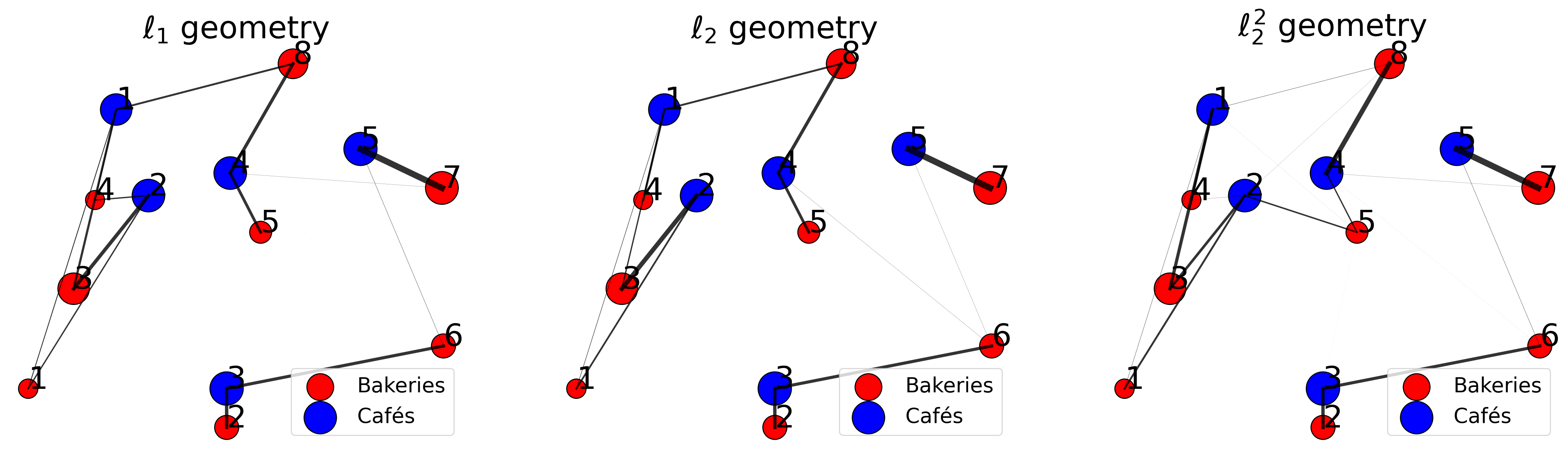
The above transport plans are obtained for \(\epsilon = 0.1 \cdot \bar{C}\). Let’s increase epsilon to \(\epsilon = 10 \cdot \bar{C}\) and replot the optimal transport plans to visualize the effect of epsilon.
# l1 geometry
epsilon = 10 * np.mean(C_l1)
optimal_plan_sinkhorn_l1_croissant, optimal_cost_sinkhorn_l1_croissant = compute_transport_sinkhorn(
    C=C_l1,
    a=bakery_prod,
    b=cafe_prod,
    epsilon=epsilon,
    verbose=False,
)

# l2 geometry
epsilon = 10 * np.mean(C_l2)
optimal_plan_sinkhorn_l2_croissant, optimal_cost_sinkhorn_l2_croissant = compute_transport_sinkhorn(
    C=C_l2,
    a=bakery_prod,
    b=cafe_prod,
    epsilon=epsilon,
    verbose=False
)

# squared l2 geometry
epsilon = 10 * np.mean(C_l2_sq)
optimal_plan_sinkhorn_l2_sq_croissant, optimal_cost_sinkhorn_l2_sq_croissant = compute_transport_sinkhorn(
    C=C_l2_sq,
    a=bakery_prod,
    b=cafe_prod,
    epsilon=epsilon,
    verbose=False
)

fig, ax = plt.subplots(
    1, 3, figsize=(9*3, 7)
)
plans = [optimal_plan_l1_croissant,
         optimal_plan_l2_croissant,
         optimal_plan_l2_sq_croissant]
titles = [r"$\ell_1$ geometry", r"$\ell_2$ geometry", r"$\ell_2^2$ geometry"]

for axes, plan, title in zip(ax, plans, titles):
  plot_assignement(
      ax=axes,
      x=bakery_pos, a=bakery_prod, x_label="Bakeries",
      y=cafe_pos, b=cafe_prod, y_label="Cafés",
      optimal_plan=plan,
      title=title
  )
plt.show()
early termination: 10
early termination: 10
early termination: 10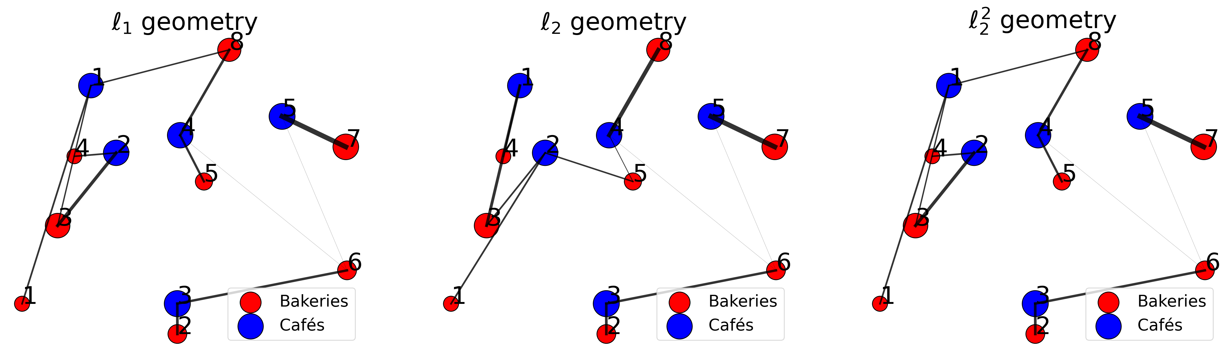
Note: If the epsilon is large, the distribution is close to uniform.
Question: What do you observe in relation to the transport plans obtained for the exact optimal transport?
Answer:
We now show that this Sinkhorn algorithm is consistent with classical optimal transport, using the “croissant” transport example and focusing on the \(\ell_2\) cost.
Question: Complete the following code to compute, for various \(\epsilon'\), values on a regular grid: * Set \(\epsilon = \epsilon' \cdot \bar{C}\), * The deviation of the entropic optimal plan \(P^*_\epsilon\) to the exact optimal plan \(P^*\), namely \(\|P^*_\epsilon - P^*\|_2\). * The deviation of the entropic optimal cost \(\langle C, P^*_\epsilon \rangle\) to the exact optimal plan \(\langle C, P^*_\epsilon \rangle\), namely: \(\langle C, P^*_\epsilon \rangle - \langle C, P^* \rangle\).
We remind that the excat optimal transport plan for the \(\ell_2\) cost is stored as variable optimal_plan_l2_croissant.
Answer:
plan_diff = []
distance_diff = []
grid = np.linspace(0.01, 5, 100)
for epsilon_prime in grid:
epsilon = epsilon_prime * np.mean(C_l2)
optimal_plan_sinkhorn_l2_croissant, optimal_cost_sinkhorn_l2_croissant = compute_transport_sinkhorn(
C=C_l2,
a=bakery_prod,
b=cafe_prod,
epsilon=epsilon,
verbose=False
)
assert optimal_cost_sinkhorn_l2_croissant != np.nan, (
"Optimal cost is nan due to numerical instabilities."
)
plan_diff.append(
np.sum(np.abs(optimal_plan_sinkhorn_l2_croissant - optimal_plan_l2_croissant))
)
distance_diff.append(
optimal_cost_sinkhorn_l2_croissant - optimal_cost_l2_croissant
)early termination: 2460
early termination: 220
early termination: 50
early termination: 30
early termination: 20
early termination: 20
early termination: 10
early termination: 10
early termination: 10
early termination: 10
early termination: 10
early termination: 10
early termination: 10
early termination: 10
early termination: 10
early termination: 10
early termination: 10
early termination: 10
early termination: 10
early termination: 10
early termination: 10
early termination: 10
early termination: 10
early termination: 10
early termination: 10
early termination: 10
early termination: 10
early termination: 10
early termination: 10
early termination: 10
early termination: 10
early termination: 10
early termination: 10
early termination: 10
early termination: 10
early termination: 10
early termination: 10
early termination: 10
early termination: 10
early termination: 10
early termination: 10
early termination: 10
early termination: 10
early termination: 10
early termination: 10
early termination: 10
early termination: 10
early termination: 10
early termination: 10
early termination: 10
early termination: 10
early termination: 10
early termination: 10
early termination: 10
early termination: 10
early termination: 10
early termination: 10
early termination: 10
early termination: 10
early termination: 10
early termination: 10
early termination: 10
early termination: 10
early termination: 10
early termination: 10
early termination: 10
early termination: 10
early termination: 10
early termination: 10
early termination: 10
early termination: 10
early termination: 10
early termination: 10
early termination: 10
early termination: 10
early termination: 10
early termination: 10
early termination: 10
early termination: 10
early termination: 10
early termination: 10
early termination: 10
early termination: 10
early termination: 10
early termination: 10
early termination: 10
early termination: 10
early termination: 10
early termination: 10
early termination: 10
early termination: 10
early termination: 10
early termination: 10
early termination: 10
early termination: 10
early termination: 10
early termination: 10
early termination: 10
early termination: 10
early termination: 10Now, let’s plot the results.
fig, ax = plt.subplots(2, 1, figsize=(16, 5*2))
reg_strengths = np.mean(C_l2) * grid
plot_consistency(
    ax,
    reg_strengths,
    plan_diff,
    distance_diff
)

plt.show()
/opt/homebrew/lib/python3.12/site-packages/IPython/core/pylabtools.py:170: UserWarning: Data has no positive values, and therefore cannot be log-scaled.
fig.canvas.print_figure(bytes_io, **kw)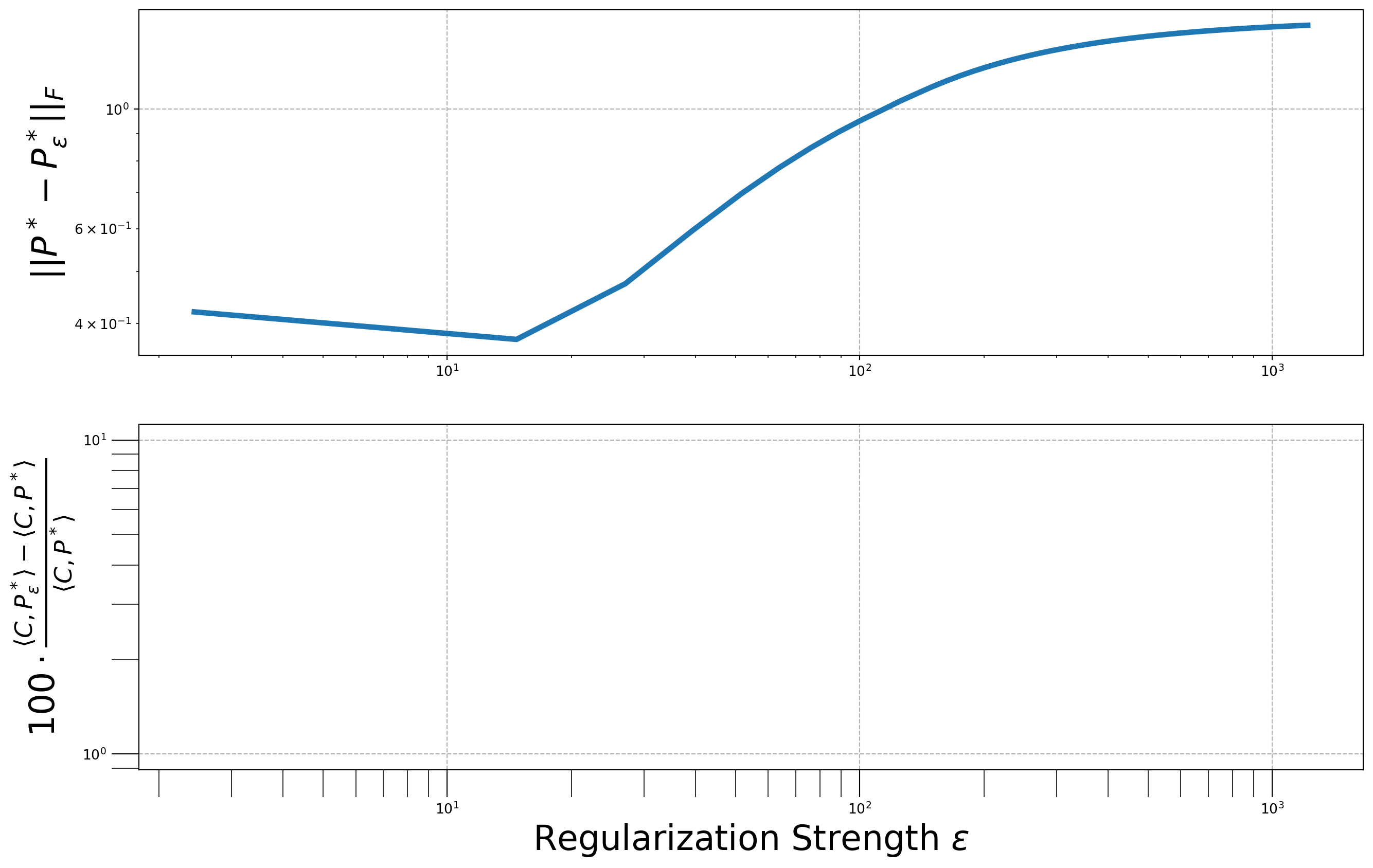
Note: The result is different from the lecturer’s.
OTT パッケージOTTFirst, you need to install OTT.
%pip install ott-jaxerror: externally-managed-environment
× This environment is externally managed
╰─> To install Python packages system-wide, try brew install
xyz, where xyz is the package you are trying to
install.
If you wish to install a Python library that isn't in Homebrew,
use a virtual environment:
python3 -m venv path/to/venv
source path/to/venv/bin/activate
python3 -m pip install xyz
If you wish to install a Python application that isn't in Homebrew,
it may be easiest to use 'pipx install xyz', which will manage a
virtual environment for you. You can install pipx with
brew install pipx
You may restore the old behavior of pip by passing
the '--break-system-packages' flag to pip, or by adding
'break-system-packages = true' to your pip.conf file. The latter
will permanently disable this error.
If you disable this error, we STRONGLY recommend that you additionally
pass the '--user' flag to pip, or set 'user = true' in your pip.conf
file. Failure to do this can result in a broken Homebrew installation.
Read more about this behavior here: <https://peps.python.org/pep-0668/>
note: If you believe this is a mistake, please contact your Python installation or OS distribution provider. You can override this, at the risk of breaking your Python installation or OS, by passing --break-system-packages.
hint: See PEP 668 for the detailed specification.
Note: you may need to restart the kernel to use updated packages.Then we load the required pakages.
import jax
import jax.numpy as jnp
import jax.random as random
import ott
from ott.geometry import costs, pointcloud
from ott.problems.linear import linear_problem
from ott.solvers.linear import sinkhornOTT and JAXOTT is a python library that allows to compute and differentiate the entropic optimal transport. In this lab session, we will focus on entropic optimal transport computation, and not differentiation. differentiation will be takcled later.
OTT is based on JAX, a package similar to PyTorch or TensorFlow, which allows to do automatic differentiation and GPU programming. It also provides useful primitives for efficient computation, such as the just-in-time (jit) compilation or the automatic vectorization map vmap. For more informations on JAX, see the tutorial https://jax.readthedocs.io/en/latest/notebooks/quickstart.html.
Unlike PyTorch or TensorFlow, JAX is very close to numpy thanks to the jax.numpy package, which implements most of the numpy features, but for the JAX data structures. For this lab session, you only need to know how to manipulate jax.numpy Arrays and generate random numbers with jax.random.
First, let’s have a look to jax.numpy and see that it works (almost) exactly as numpy. Usually, one imports jax.numpy as jnp as done in the above cells, and developp as with numpy, by just replacing np by jnp. Note that jax.numpy Arrays are called DeviceArray. For more informations on jax.numpy, see https://jax.readthedocs.io/en/latest/jax-101/01-jax-basics.html.
d = 5
u = 5 * jnp.ones(5)
Id = jnp.eye(5)
print(type(u))
print(f"u = {u}")
print(f"Id = {Id}")
print(f"Id @ u = {jnp.dot(Id, u)}")
print(f"sum(u) = {jnp.sum(u)}")
print(f"var(u) = {jnp.var(u)}")
<class 'jaxlib.xla_extension.ArrayImpl'>
u = [5. 5. 5. 5. 5.]
Id = [[1. 0. 0. 0. 0.]
[0. 1. 0. 0. 0.]
[0. 0. 1. 0. 0.]
[0. 0. 0. 1. 0.]
[0. 0. 0. 0. 1.]]
Id @ u = [5. 5. 5. 5. 5.]
sum(u) = 25.0
var(u) = 0.0With numpy.random, you can generate random numbers on the fly without giving the seed. For example, np.random.rand() generates a random number \(x \sim U([0, 1])\). Indeed, numpy.random uses an internal seed which is updated each time a random number generating function is called. On the other hand, with jax.random, we must give the seed each time we generate random numbers. To some extent, we want to always control the randomness. Moreover, we do not pass exactly a seed but a jax.random.PRNGKey key which is itself instantiated from a seed. Let’s see it on an example.
rng = jax.random.PRNGKey(0)
n, d = 13, 2
x = jax.random.normal(rng, (n, d))
print(f"x = {x}")
x = [[ 2.516351 -1.3947194 ]
[-0.8633262 0.6413567 ]
[-0.37789643 -0.6044598 ]
[ 1.9069 -0.17918469]
[-0.7583423 -0.5160155 ]
[ 1.2666148 -0.12342127]
[ 0.28430256 -0.17251171]
[ 1.0661486 1.5814103 ]
[-2.0284636 -0.13168257]
[-0.14515765 0.21532312]
[-0.69525063 -0.9314128 ]
[-0.89809936 -0.25272107]
[-0.34937173 1.8394127 ]]Then, to have new keys to generate new random numbers, we need to split the key via jax.random.split, which generate \(n \geq 2\) new keys from a key.
rng1, rng2, rng3 = jax.random.split(rng, 3)
a = jax.random.normal(rng1, (n, d))
b = jax.random.normal(rng2, (n, d))
c = jax.random.normal(rng2, (n, d))
print(f"a = {a}")
print(f"b = {b}")
print(f"c = {c}")
a = [[-0.38696066 -0.96707183]
[ 1.0078175 -0.6096286 ]
[-1.153353 1.0749092 ]
[-1.2452031 -0.63885343]
[ 0.01121208 0.2842425 ]
[ 0.5296049 0.26609063]
[ 0.8728492 1.0844501 ]
[ 1.4472795 -0.82503337]
[-0.41826957 0.21321987]
[ 1.9602116 0.17687395]
[-0.9978761 -2.0551765 ]
[-0.4094941 -1.4577458 ]
[-1.0969195 -0.66684234]]
b = [[ 0.10911155 -0.45371595]
[ 0.12062439 -0.06927001]
[ 0.00600028 2.3732579 ]
[-0.17656058 1.7653493 ]
[-0.06429235 0.487175 ]
[-1.1079016 -1.0277865 ]
[-0.0553451 -0.28271845]
[-0.9633478 -0.05370665]
[ 0.20281292 -0.16658288]
[ 0.8015828 -0.61697495]
[-0.30176872 -1.1862007 ]
[-3.106658 -0.03262986]
[ 0.53711027 0.21359496]]
c = [[ 0.10911155 -0.45371595]
[ 0.12062439 -0.06927001]
[ 0.00600028 2.3732579 ]
[-0.17656058 1.7653493 ]
[-0.06429235 0.487175 ]
[-1.1079016 -1.0277865 ]
[-0.0553451 -0.28271845]
[-0.9633478 -0.05370665]
[ 0.20281292 -0.16658288]
[ 0.8015828 -0.61697495]
[-0.30176872 -1.1862007 ]
[-3.106658 -0.03262986]
[ 0.53711027 0.21359496]]you now know everything you need for the moment!
OTTNow let’s use the implementation of the OTT Sinkhorn algorithm, on some random weighted point clouds. Then you will, by yourself, use it on the “croissant” transport example.
Let’s first generate the data.
# generate data
rng = jax.random.PRNGKey(0)
rng1, rng2 = jax.random.split(rng, 2)
n, m, d = 13, 17, 2
x = jax.random.normal(rng1, (n, d))
y = jax.random.normal(rng2, (m, d)) + 1
a = jnp.ones(n) / n
b = jnp.ones(m) / m
Then, we have to define a PointCloud geometry which contains: * the point clouds x and y, * the cost function cost_fn, * the entropic regularization strength epsilon.
Note that the geometry does not contain the weight vectors a and b, these are passed later.
The cost_fn should be an istance of ott.geometry.CostFn. Most of the usual costs are implemented. For example, the three costs \(\ell_1, \ell_2\) and \(\ell_2^2\) are implemented. Here, we will focus on the \(\ell_2\) cost, implemented by ott.geometry.costs.Euclidean. See https://ott-jax.readthedocs.io/en/latest/_autosummary/ott.geometry.costs.CostFn.html#ott.geometry.costs.CostFn for more information on the provided cost_fn.
We still choose epsilon to be \(0.1 \cdot \bar{C}\). To do this, we set relative_epsilon=True when instantiating the geometry. The term relative means that epsilon is chosen relatively to the mean of the cost matrix. Passing then epsilon=0.1, the value of epsilon used by Sinkhorn will be \(0.1 \cdot \bar{C}\).
# define geometry
geom = pointcloud.PointCloud(
    x=x, y=y,
    cost_fn=costs.Euclidean(),
    epsilon=1e-1,
    relative_epsilon=True
)
We then define an optimization problem from this geometry, which is the problem we will solve with the Sinkhorn algorithm. We instantiate this optimization problem as an object of the class linear_problem.LinearProblem. We pass the weight vectors a and b because they define the constraints of the linear problem. Then, we instantiate a Sinkhorn solver, object of the class sinkhorn.Sinkhorn, which we will use to solve this optimization problem.
The OTT library is designed in this way because it allows to solve other optimal transport problems, which do not necessarily have a linear problem structure, and which use other solvers than Sinkhorn.
# create optimization problem
ot_prob = linear_problem.LinearProblem(geom, a=a, b=b)

# create sinkhorn solver
solver = sinkhorn.Sinkhorn(ot_prob)

# solve the OT problem
ot_sol = solver(ot_prob)
The ot output object contains several callables and properties, notably a boolean assessing the Sinkhorn convergence, the marginal errors throughtout iterations and the optimal transport plan.
print(
    " Sinkhorn has converged: ",
    ot_sol.converged,
    "\n",
    "Error upon last iteration: ",
    ot_sol.errors[(ot_sol.errors > -1)][-1],
    "\n",
    "Sinkhorn required ",
    jnp.sum(ot_sol.errors > -1),
    " iterations to converge. \n",
    "entropic OT cost: ",
    jnp.sum(ot_sol.matrix * ot_sol.geom.cost_matrix),
)
Sinkhorn has converged: True
Error upon last iteration: 0.00019063428
Sinkhorn required 5 iterations to converge.
entropic OT cost: 29.436863Question: Compute the entropic optimal transport plan and cost for the “croissant” transport problem, with \(\ell_2\) cost and \(\epsilon = 0.1 \cdot \bar{C}\). Then, plot the optimal transport plan.
Answer:
Marco Cuturi による Colab を参考にした.
