流体モデル概観 – Hirofumi Shiba

概要

Lorenz’ 63, Lorenz’ 96 とはそれぞれ (Lorenz, 1963), (Lorenz, 1995) によって導入された大気モデルである．前者はバタフライ効果の語源ともなった，最初に特定されたカオス力学系でもある． Navier-Stokes 方程式は流体の運動を記述する方程式である．これらはいずれもデータ同化・軌道推定技術のベンチマークとして用いられている．ここでそれぞれのモデルの数学的性質と Julia を通じたシミュレーションの方法をまとめる．

Loorenz96.jl パッケージ (K, 2021)
DynamicalSystems.jl (GitHub / Docs) パッケージ
EnsembleKalmanProcesses.jl (GitHub / Docs) パッケージ

1 Lorenz 96 モデル

1.1 モデル定義

Lorenz 96 とは，(Lorenz, 1995) によって導入された力学系の通称である：

\[ \frac{d x_i}{d t}=\biggr(x_{i+1}-x_{i-2}\biggl)x_{i-1}-x_i+F,\qquad F\in\mathbb{R}. \]

ただし，係数については，空間の次元 \(x\in\mathbb{R}^N\) について \(x_{i-N}=x_{i+N}=x_i\) と約束する．

1.2 `DynamicalSystems.jl` でシミュレーション

DynamicalSystems.jl (GitHub / Docs) パッケージのチュートリアルに Lorenz96 の例がある．

\(F=8\) の場合はカオス的な振る舞いを示す：

using DynamicalSystems

function lorenz96_rule!(du, u, p, t)
    F = p[1]; N = length(u)
    # 3 edge cases
    du[1] = (u[2] - u[N - 1]) * u[N] - u[1] + F
    du[2] = (u[3] - u[N]) * u[1] - u[2] + F
    du[N] = (u[1] - u[N - 2]) * u[N - 1] - u[N] + F
    # then the general case
    for n in 3:(N - 1)
        du[n] = (u[n + 1] - u[n - 2]) * u[n - 1] - u[n] + F
    end
    return nothing # always `return nothing` for in-place form!
end

N = 6
u0 = range(0.1, 1; length = N)
p0 = [8.0]
lorenz96 = CoupledODEs(lorenz96_rule!, u0, p0)

total_time = 12.5
sampling_time = 0.02
Y, t = trajectory(lorenz96, total_time; Ttr = 2.2, Δt = sampling_time)

(6-dimensional StateSpaceSet{Float64} with 626 points, 2.2:0.02:14.7)

using Plots

p = plot(xlabel = "time", ylabel = "variable", legend = false)
for var in eachcol(Y)
    plot!(p, t, var)
end
plot(p)

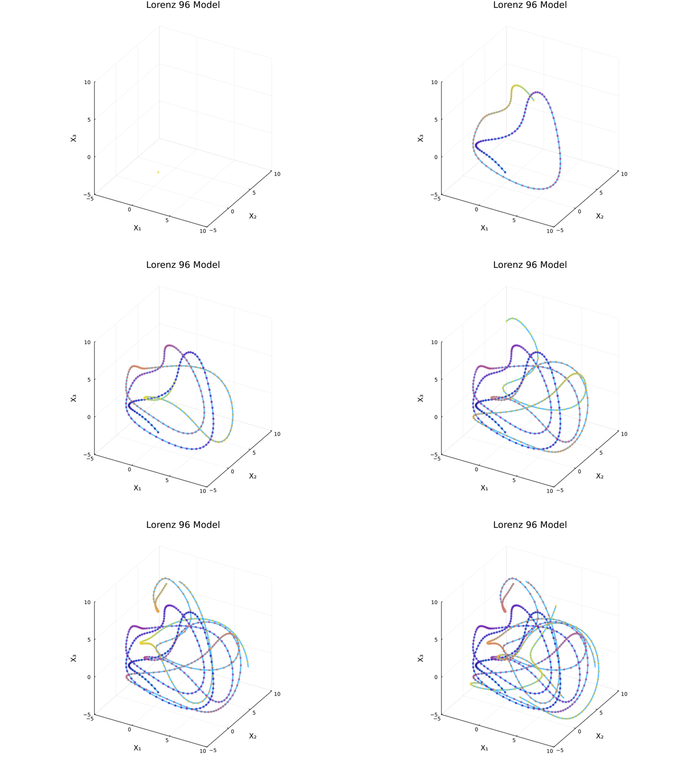
最初の３成分を取り出して，３次元空間にプロットしてみる：¹

ODE ソルバーの選択

CoupledODEs のデフォルトのソルバーは

Tsit5 - Tsitouras 5/4 Runge-Kutta method. (free 4th order interpolant).

である (Tsitouras, 2011)．次のようにカスタマイズもできる

using OrdinaryDiffEq: Vern9 # accessing the ODE solvers
diffeq = (alg = Vern9(), abstol = 1e-9, reltol = 1e-9)
lorenz96_vern = ContinuousDynamicalSystem(lorenz96_rule!, u0, p0; diffeq)

Y, t = trajectory(lorenz96_vern, total_time; Ttr = 2.2, Δt = sampling_time)
Y[end]

1.3 ２タイムスケール版

(Section 4 Lorenz, 1995) では２タイムスケール版の Lorenz 96 モデルが導入されている： \[\begin{align*} \frac{d x_i}{d t}&=-x_{i-1}(x_{i-2}-x_{i+1})-x_i+F-\left(\frac{hc}{b}\right)\sum_{j=1}^{J-1}Y_{j,i},\\ \frac{d y_{j,i}}{d t}&=-cbY_{j+1,i}(Y_{j+2,i}-Y_{j-1,i})-cY_{j,i}+\frac{hc}{b}X_i. \end{align*}\]

2 非圧縮・粘性 Navier-Stokes 方程式

2.1 モデル定義

\(M^n\) を \(n\)-次元可微分多様体，\(v:M\times\mathbb{R}_+\to\mathbb{R}^n\) を \(M\) 上のベクトル場とする．\(v\) に関する非圧縮・粘性 Navier-Stokes 方程式は次のように表せる (Temam, 1995), (Evans, 2010, p. 6)：

\[ \partial_tv-\nu\mathop{}\!\mathbin\bigtriangleup v+v\cdot\nabla v=f-\nabla p,\qquad\nu>0, \] \[ \operatorname{div}v=0,\quad\int_M v_j(x,-)\,dx=0\quad(j\in[n]),\quad v(x,0)=:u(x). \] \(\nu>0\) を粘性 (viscosity) 係数，\(p:M\times\mathbb{R}_+\to\mathbb{R}\) を圧力 (pressure) という．\(f\) は時間一定の外力である．²

2.2 数値解法

周期的境界条件

\(M^n=:\Omega\) を \(\mathbb{R}^n\) の領域とし，周期的な境界条件 \[ v(x+Le_i,t)=v(x,t),\qquad(x,t)\in M^n\times\mathbb{R}_+ \] を考える．ただし，\(e_i\) は \(\mathbb{R}^n\) の標準基底ベクトルである．

この設定の下では数学的に理想的な取り扱いができる．物理的には例えばトーラス上の流体を考えていることに相当する．

\(v\) を数値的に得るためには 射影法 (projection method) (Chorin, 1967), (Chorin, 1968) を用いる．

この方法では Helmholtz-Hodge の射影作用素 \(P\) が用いられる．

これは \[ \frac{d v}{d t}+\nu Av+B(v,v)=P(f),\qquad v(0)=u \tag{1}\] という（無限次元空間 \(v\in V'\) 上の） ODE への帰着を可能にする．ただし， \[ B(v,w):=\frac{1}{2}P(v\cdot\nabla w)+\frac{1}{2}P(w\cdot\nabla v). \]

あとは ODE (1) をソルバーで解くのである．

2.3 数学的詳細³

\(H^m(\Omega)\subset L^2(\Omega)\) を \(m\) 階までの導関数が全て \(L^2(\Omega)\) に属する関数からなる Sobolev 空間とする．

\(H_p^m(\Omega)\) を \(H_\mathrm{loc}^m(\mathbb{R}^n)\) の部分空間のうち，\(\Omega\) 上で周期的なものとすると，次の表示を持つ： \[ H_p^m(\Omega)=\left\{u=\sum_{k\in\mathbb{Z}^n}c_ke^{2i\pi k\cdot x/L}\,\middle|\,\overline{c}_k=c_{-k},\sum_{k\in\mathbb{Z}^n}\lvert k\rvert^{2m}\lvert c_k\rvert^2<\infty\right\}. \] \(\dot{H}_p^m(\Omega)\) を \(H_p^m(\Omega)\) のうち \(c_0=0\) を満たすものの部分空間とする．上の表示をもとにして，任意の \(m\in\mathbb{R}\) について \(\dot{H}^m_p(\Omega)\) が定まる．

\[ V:=\left\{u\in H^1_p(\Omega)\,\middle|\,\operatorname{div}u=0\,\mathrm{on}\;\mathbb{R}^n\right\},\qquad H:=\left\{u\in H^0_p(\Omega)\,\middle|\,\operatorname{div}u=0\,\mathrm{on}\;\mathbb{R}^n\right\} \] について \(V\subset H\subset V^*\) が成り立つ．

以上の設定では，\(A:V\overset{\sim}{\to}V^*\) は同型，\(B:V\times V\hookrightarrow V^*\) は連続な双線型作用素になる．

\(P\) は Helmholtz 射影と呼ばれ，\(V^*\) 上への射影を与える．⁴

2.4 Galerkin 近似

\(A\) の固有関数を \((w_i)\) とし，最初の \(m\) 個の固有関数が定める空間上への射影を \(P_m\) とし， \[ \frac{d v_m}{d t}+\nu Av_m+P_mB(v_m)=P_mf,\qquad t>0,v_m(0)=P_mv_0. \] を解く．この \(v_m\) を \(v\) の Galerkin 近似 という (Temam, 1995, p. 109)．

こうして得る有限次元空間上の ODE はまだ 硬い方程式 であり，例えば指数的な有限差分を取る (Cox and Matthews, 2002) などの処置が必要である．

(Section 5 Kantas et al., 2014) はデータ同化の文脈でこれを解いている．

2.5 シミュレーション

IncompressibleNavierStokes.jl (GitHub / Docs) パッケージを用いて，非圧縮 Navier-Stokes 方程式を解くことができる．

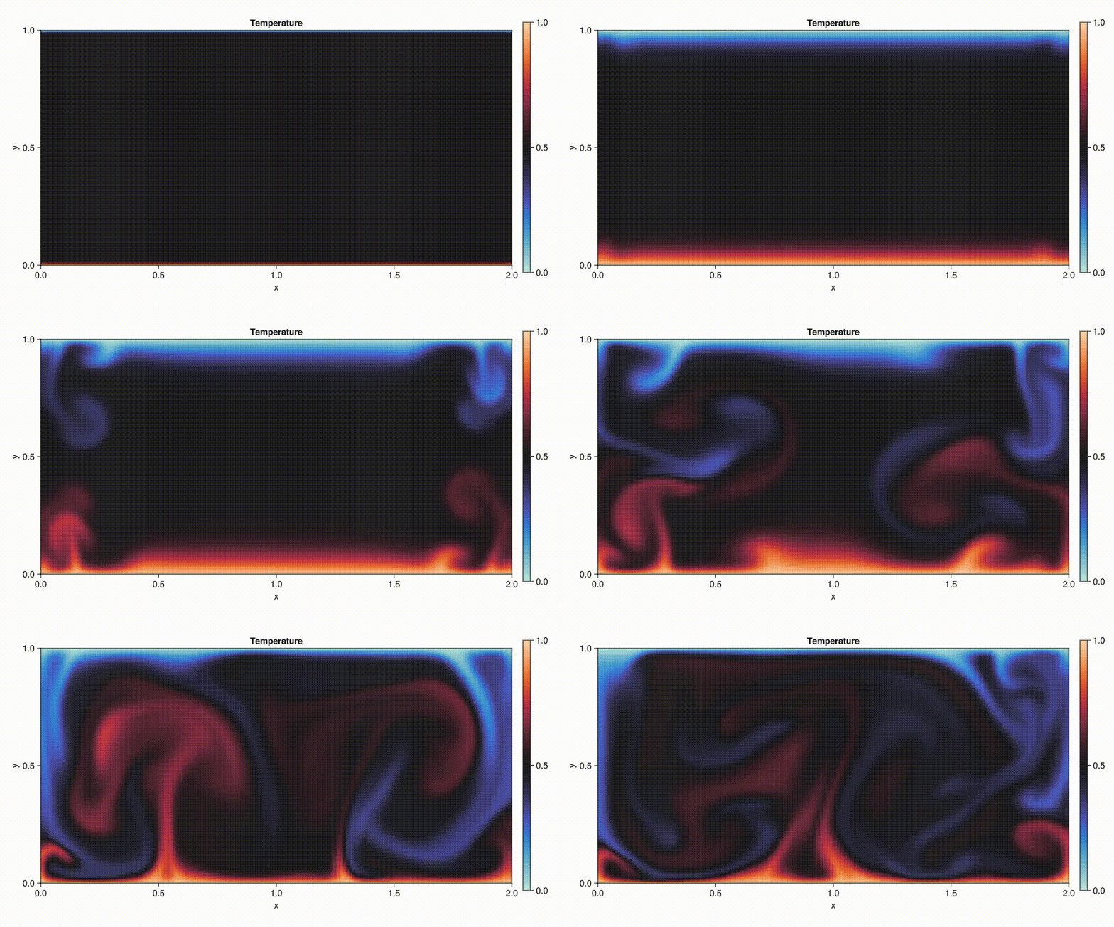
Rayleigh-Bénard 対流問題を実行するサンプルコードが提示されている．

Rayleigh-Bénard 対流は二次元空間を下から加熱した際の流体の対流で，Bénard 細胞と呼ばれる散逸構造が現れるはずである．

using GLMakie
using IncompressibleNavierStokes

# Setup
setup = Setup(
    x = (tanh_grid(0.0, 2.0, 200, 1.2), tanh_grid(0.0, 1.0, 100, 1.2)),
    boundary_conditions = ((DirichletBC(), DirichletBC()), (DirichletBC(), DirichletBC())),
    temperature = temperature_equation(;
        Pr = 0.71,
        Ra = 1e7,
        Ge = 1.0,
        boundary_conditions = (
            (SymmetricBC(), SymmetricBC()),
            (DirichletBC(1.0), DirichletBC(0.0)),
        ),
    ),
)

# Solve equation
solve_unsteady(;
    setup,
    ustart = velocityfield(setup, (dim, x, y) -> zero(x)),
    tempstart = temperaturefield(setup, (x, y) -> 1 / 2 + sinpi(30 * x) / 100),
    tlims = (0.0, 30.0),
    Δt = 0.02,
    processors = (;
        anim = animator(;
            setup,
            path = "temperature.mp4",
            fieldname = :temperature,
            colorrange = (0.0, 1.0),
            size = (900, 500),
            colormap = :seaborn_icefire_gradient,
            nupdate = 5,
        ),
    ),
)

solve_unsteady() 関数は method = RKMethods.RK44(; T = eltype(ustart[1])), がデフォルトである．

RK44 は 4 次の Runge-Kutta 法である．４次の Runge-Kutta 法は圧力に懸念があることを除いて，速度場の解法としては悪くない性能を示すようである (Sanderse and Koren, 2012)．

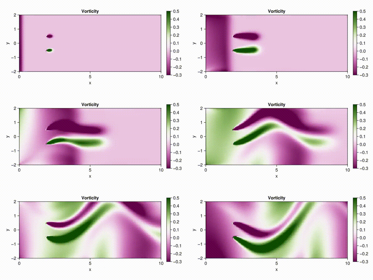
例えば非一様な風が障害物に当たる場合のシミュレーション例では，圧力も２次まで計算する RK44P2() を用いている．

using IncompressibleNavierStokes

n = 40
x = LinRange(0.0, 10.0, 5n + 1), LinRange(-2.0, 2.0, 2n + 1)
plotgrid(x...; figure = (; size = (600, 300)))

inflow(dim, x, y, t) = sinpi(sinpi(t / 6) / 6 + (dim == 1) / 2)
boundary_conditions = ((DirichletBC(inflow), PressureBC()), (PressureBC(), PressureBC()))

xc, yc = 2.0, 0.0 # Disk center
D = 1.0           # Disk diameter
δ = 0.11          # Disk thickness
C = 0.2           # Thrust coefficient
c = C / (D * δ)   # Normalize
inside(x, y) = abs(x - xc) ≤ δ / 2 && abs(y - yc) ≤ D / 2
bodyforce(dim, x, y, t) = -c * (dim == 1) * inside(x, y)

setup = Setup(; x, Re = 100.0, boundary_conditions, bodyforce, issteadybodyforce = true);

ustart = velocityfield(setup, (dim, x, y) -> inflow(dim, x, y, 0.0))

state, outputs = solve_unsteady(;
    setup,
    ustart,
    tlims = (0.0, 12.0),
    method = RKMethods.RK44P2(),
    Δt = 0.05,
    processors = (
        anim = animator(;
            setup,
            path = "navier_stokes_animation.mp4",
            fieldname = :vorticity,
            colorrange = (-0.3, 0.5),
            size = (600, 300),
            colormap = :bam,
            nupdate = 5,
        ),
        log = timelogger(; nupdate = 24),
    ),
);

blade の両端で過度が生じていることがわかる．

3 文献紹介

(van/ Kekem, 2018), (Kerin and Engler, 2022) が概観に良い．(Balwada and Zanna, 2023) は２タイムスケール版について詳しい．

Navier-Stokes 方程式のデータ同化に関しては (Kantas et al., 2014) などで考えられている．

References

Balwada, A., D., and Zanna, L. (2023). Learning Machine Learning with Lorenz-96. Authorea Preprints.

Chorin, A. J. (1967). The numerical solution of the Navier-Stokes equations for an incompressible fluid. Bulletin of the American Mathematical Society, 73(6), 928–931.

Chorin, A. J. (1968). Numerical solution of the navier-stokes equations. Mathematics of Computation, 22(104), 745–762.

Cox, S. M., and Matthews, P. C. (2002). Exponential time differencing for stiff systems. Journal of Computational Physics, 176(2), 430–455.

Evans, L. C. (2010). Partial differential equations,Vol. 19. American Mathematical Society.

K, M. (2021, July). Milankl/Lorenz96.jl: v0.3.0 (Version v0.3.0). Zenodo.

Kantas, N., Beskos, A., and Jasra, A. (2014). Sequential monte carlo methods for high-dimensional inverse problems: A case study for the navier–stokes equations. SIAM/ASA Journal on Uncertainty Quantification, 2(1), 464–489.

Kerin, J., and Engler, H. (2022). On the lorenz ’96 model and some generalizations. Discrete and Continuous Dynamical Systems - B.

Lorenz, E. N. (1963). Deterministic nonperiodic flow. Journal of Atmospheric Sciences, 20(2), 130–141.

Lorenz, E. N. (1995). Predictability: A problem partly solved. In Seminar on predictability, 4-8 september 1995. ECMWF.

Sanderse, B., and Koren, B. (2012). Accuracy analysis of explicit runge–kutta methods applied to the incompressible navier–stokes equations. Journal of Computational Physics, 231(8), 3041–3063.

Temam, R. M. (1995). Navier–stokes equations and nonlinear functional analysis. Society for Industrial; Applied Mathematics.

Tsai, T.-P. (2018). Lectures on navier-stokes equations,Vol. 192. American Mathematical Society.

Tsitouras, Ch. (2011). Runge–kutta pairs of order 5(4) satisfying only the first column simplifying assumption. Computers & Mathematics with Applications, 62(2), 770–775.

van/ Kekem, D. L. (2018). Dynamics of the lorenz-96 model: Bifurcations, symmetries and waves (PhD thesis). University of Groningen. Retrieved from https://research.rug.nl/en/publications/dynamics-of-the-lorenz-96-model-bifurcations-symmetries-and-waves

Footnotes

コードはこちらを参照．↩︎
上述の方程式は，係数を正規化した場合とも，正規化した関数に関する方程式とも解釈できる．後者の解釈では，\(\nu^{-1}\) は Reynolds 数に対応する．↩︎
本小節は (Section 2 Temam, 1995) を参考にしている．↩︎
(Tsai, 2018, p. 16) も参照．↩︎