YUIMA 入門
2024-05-17
yuima は確率過程のモデリングとその統計推測を可能にするフレームワークです.広範なクラスの確率微分方程式のシミュレーションが可能です.今回はこのような確率過程に対する統計推測を実行する方法を紹介します.yuima は従来の i.i.d. 仮定の下での統計推測から,一般の確率過程の統計推測への橋渡しを目標としています.ほとんどの手法が,\(N\to\infty,\Delta_n\to0\) の極限で得られるデータ(高頻度データ)にも応用可能な手法となっています.
A Blog Entry on Bayesian Computation by an Applied Mathematician
$$
$$
setYuimaコンストラクタsetYuima(data, model, sampling, characteristic, functional)data を yuima オブジェクトに持たせた場合,データからパラメータ推定を行うことができる.
data <- read.csv("http://chart.yahoo.com/table.csv?s=IBM&g=d&x=.csv")
x <- setYuima(data = setData(data$Close))
str(x@data)\(r\)-次元 Wiener 過程 \(\{W_t\}\) が定める拡散過程 \[ dX_t=a(X_t,\theta_2)\,dt+b(X_t,\theta_1)\,dW_t \] のパラメータ \(\theta_1\in\Theta_1\subset\mathbb{R}^p,\theta_2\in\Theta_2\subset\mathbb{R}^q\) の推定を考えたい.
データ \[ \boldsymbol{X}_n:=(X_{t_i})_{i=0}^n,\qquad t_i:=i\Delta_n \] の対数尤度は次の 擬似対数尤度 を用いて近似できる: \[ \ell_n(\boldsymbol{X}_n,\theta)=-\frac{1}{2}\sum_{i=1}^n\left(\log\det(\Sigma_{i-1}(\theta_1))+\frac{1}{\Delta_n}\Sigma_{i-1}^{-1}(\theta_1)\biggr((\Delta X_i-\Delta_na_{i-1}(\theta_2))^{\otimes 2}\biggl)\right) \] ただし \[ \Delta X_i:=X_{t_i}-X_{t_{i-1}},\quad\Sigma_i(\theta_1):=\Sigma(\theta_1,X_{t_i}) \] \[ a_i(\theta_2):=a(X_{t_i},\theta_2),\quad\Sigma:=b^{\otimes2},\quad A^{\otimes2}:=AA^\top \] とした.
この擬似対数尤度 \(\ell_n(\boldsymbol{X}_n,\theta)\) を用いて, \[ \widehat{\theta}:=\operatorname*{argmax}_{\theta}\ell_n(\boldsymbol{X}_n,\theta) \] と定まる \(M\)-推定量を 擬似最尤推定量 という.
これを実装する qmle 関数が, stats4 標準の mle 関数 に似せて作られている.
qmle(yuima, start, method = "L-BFGS-B", fixed = list(), print = FALSE, envir = globalenv(), lower, upper, joint = FALSE, Est.Incr ="NoIncr", aggregation = TRUE, threshold = NULL, rcpp =FALSE, ...)start は最適化を始める初期値を,名前に対応づける辞書の形で与える.yuima オブジェクトは model と data のスロットが埋められていなければならない.最適化は BFGS によって行われる.
ジャンプ過程への応用も今後予定されている.
例えば,次のモデル \[ dX_t=(2-\theta_2X_t)dt+(1+X_t^2)^{\theta_1}dW_t,\quad X_0=1, \] を考え,真値を \(\theta_1=0.2,\theta_2=0.3\) としてデータを生成する.
library(yuima)
ymodel <- setModel(drift="(2-theta2*x)", diffusion="(1+x^2)^theta1")
n <- 750
ysamp <- setSampling(Terminal=n^(1/3), n=n)
yuima <- setYuima(model=ymodel, sampling=ysamp)
yuima <- simulate(yuima, xinit=1, true.parameter=list(theta1=0.2, theta2=0.3))
これに対して,QMLE を実行してみる:
param.init <- list(theta2=0.5, theta1=0.5)
low.par <- list(theta1=0, theta2=0)
upp.par <- list(theta1=1, theta2=1)
mle1 <- qmle(yuima, start=param.init, lower=low.par, upper=upp.par)
summary(mle1)
Quasi-Maximum likelihood estimation
Call:
qmle(yuima = yuima, start = param.init, lower = low.par, upper = upp.par)
Coefficients:
Estimate Std. Error
theta1 0.1785256 0.01337509
theta2 0.8495606 0.19301758
-2 log L: -708.956 \(\theta_2\) の推定の方が圧倒的に難しいらしいことがよくわかる.
実は高頻度極限 \(\Delta_n\to0,n\to\infty\) において,\(\widehat{\theta}_1\) は漸近的に混合正規である (Genon-Catalot and Jacod, 1993).
\(\widehat{\theta}_2\) も一致性を持つには,条件 \(T=n\Delta_n\to\infty\) が必要である.これは \(T\) が有限であるとき \(\theta_2\) の Fisher 情報量も有限であり,それゆえこの設定したでは一致推定量が存在しないためである.
\(T\to\infty\) の下でエルゴード条件を仮定すれば,一致性だけでなく漸近正規性も達成される.
局所 Gauss 近似を成立させるためには \(n\Delta_n^2\to0\) が必要であるが,これでは条件が強すぎる.任意の \(p\ge2\) に対して条件 \(n\Delta_n^p\to0\) しか満たさない場合での適応的推定法が (Uchida and Yoshida, 2012) によって,大偏差原理による議論に基づいて提案された.
\(T\) が大きくない場合, \(\theta_2\) には小標本的な影響が現れる.これは適応的 Bayes 推定(第 3 節)でも議論する.
なお適応的 Bayes 事後平均推定量も,上述の \(\widehat{\theta}_1,\widehat{\theta}_2\) と全く同じ漸近的性質を持つ.
\(r\)-次元モデル
\[ dX_t=a(X_t,\theta_2)dt+b(X_t,\theta_1)dW_t \]
の擬似対数尤度
\[ \ell_n(\boldsymbol{X}_n,\theta)=-\frac{1}{2}\sum_{i=1}^n\left(\log\det(\Sigma_{i-1}(\theta_1))+\frac{1}{\Delta_n}\Sigma_{i-1}^{-1}(\theta_1)\biggr((\Delta X_i-\Delta_na_{i-1}(\theta_2))^{\otimes 2}\biggl)\right) \]
を考える.
まず,任意に初期値 \(\theta^\star_2\in\Theta_2\) を取り,\(\theta_1\) に事前分布 \(\pi_1\) を導入して,これに基づいて Bayes 事後平均推定量 を \[ \widetilde{\theta}_1:=\frac{\int_{\Theta_1}\theta_1\exp(\ell_n(\boldsymbol{X}_n,(\theta_1,\theta_2^\star)))\pi_1(\theta_1)d\theta_1}{\int_{\Theta_1}\exp(\ell_n(\boldsymbol{X}_n,(\theta_1,\theta_2^\star)))\pi_1(\theta_1)d\theta_1} \] と定める.
\(\pi_1\) が \(\Theta_1\) 全域を台に持つならば,高頻度極限で良い漸近的性質を持つことは保証される(第 2.3 節).
続いて,\(\theta_2\) に事前分布 \(\pi_2\) を導入して,\(\widetilde{\theta}_1\) から Bayes 事後平均推定量 を \[ \widetilde{\theta}_2:=\frac{\int_{\Theta_2}\theta_1\exp(\ell_n(\boldsymbol{X}_n,(\widetilde{\theta}_1,\theta_2)))\pi_2(\theta_2)d\theta_2}{\int_{\Theta_2}\exp(\ell_n(\boldsymbol{X}_n,(\widetilde{\theta}_1,\theta_2)))\pi_2(\theta_2)d\theta_2} \] と定める.
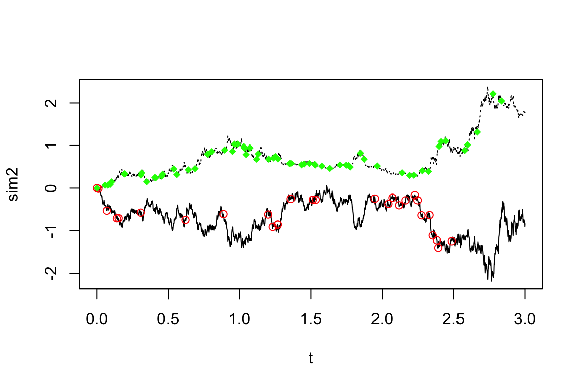
同様のモデル \[ dX_t=(2-\theta_2X_t)dt+(1+X_t^2)^{\theta_1}dW_t,\quad X_0=1, \] を考え,真値を \(\theta_1=0.2,\theta_2=0.3\) としてデータを生成する.
ymodel <- setModel(drift="(2-theta2*x)", diffusion="(1+x^2)^theta1")
n <- 750
ysamp <- setSampling(Terminal=n^(1/3), n=n)
yuima <- setYuima(model=ymodel, sampling=ysamp)
yuima <- simulate(yuima, xinit=1, true.parameter=list(theta1=0.2, theta2=0.3))
加えて,一様事前分布を用意する.
prior <- list(theta2=list(measure.type="code", df="dunif(theta2,0,1)"),
theta1=list(measure.type="code", df="dunif(theta1,0,1)"))
bayes1 <- adaBayes(yuima, start=param.init, prior=prior, mcmc=1000)
summary(mle1)Quasi-Maximum likelihood estimation
Call:
qmle(yuima = yuima, start = param.init, lower = low.par, upper = upp.par)
Coefficients:
Estimate Std. Error
theta1 0.1785256 0.01337509
theta2 0.8495606 0.19301758
-2 log L: -708.956 bayes1@coef theta1 theta2
0.1866106 0.4459654 str(bayes1)Formal class 'adabayes' [package "yuima"] with 6 slots
..@ mcmc :List of 1
.. ..$ : chr "NULL"
..@ accept_rate:List of 1
.. ..$ : chr "NULL"
..@ coef : Named num [1:2] 0.187 0.446
.. ..- attr(*, "names")= chr [1:2] "theta1" "theta2"
..@ call : language adaBayes(yuima = yuima, start = param.init, prior = prior, mcmc = 1000)
..@ vcov : num [1:2, 1:2] 0 0 0 0
..@ fullcoef : Named num [1:2] 0.187 0.446
.. ..- attr(*, "names")= chr [1:2] "theta1" "theta2"ドリフト係数 \(a(X_t,\theta_2)\) に関する推定は,\([0,T]\) の長さに強い影響を受けることが理論的にも知られている.
数値実験では \(n=750\) かつ \[ T=n^{\frac{1}{3}}\approx9.09 \] と取った.
これをさらに \(n=500,T\approx7.94\) とすると,
n <- 500
ysamp <- setSampling(Terminal=n^(1/3), n=n)
yuima <- setYuima(model=ymodel, sampling=ysamp)
yuima <- simulate(yuima, xinit=1, true.parameter=list(theta1=0.2, theta2=0.3))
mle2 <- qmle(yuima, start=param.init, lower=list(theta1=0, theta2=0), upper=list(theta1=1, theta2=1))
bayes2 <- adaBayes(yuima, start=param.init, prior=prior, mcmc=1000)summary(mle2)Quasi-Maximum likelihood estimation
Call:
qmle(yuima = yuima, start = param.init, lower = list(theta1 = 0,
theta2 = 0), upper = list(theta1 = 1, theta2 = 1))
Coefficients:
Estimate Std. Error
theta1 0.2030917 0.01011359
theta2 0.3611649 0.13888986
-2 log L: -18.11409 bayes2@coef theta1 theta2
0.2077571 0.3706500 str(bayes2)Formal class 'adabayes' [package "yuima"] with 6 slots
..@ mcmc :List of 1
.. ..$ : chr "NULL"
..@ accept_rate:List of 1
.. ..$ : chr "NULL"
..@ coef : Named num [1:2] 0.208 0.371
.. ..- attr(*, "names")= chr [1:2] "theta1" "theta2"
..@ call : language adaBayes(yuima = yuima, start = param.init, prior = prior, mcmc = 1000)
..@ vcov : num [1:2, 1:2] 0 0 0 0
..@ fullcoef : Named num [1:2] 0.208 0.371
.. ..- attr(*, "names")= chr [1:2] "theta1" "theta2"小標本でも適応的 Bayes 推定量はよく振る舞う.一方で,QMLE では劣化が激しい.\(\widehat{\theta}_1\) は小標本の影響を \(\widehat{\theta}_2\) ほどは大きく受けない.
2つの伊藤過程が非同期的に離散観測されたとして,2つの間の共分散を推定する (Hayashi and Yoshida, 2005) 推定量も yuima には実装されている.
setYuima() の help ページに ‘PLEASE FINISH THIS’ が2箇所ある.
help ページによく出てくる yuimadocs パッケージとは?
coef(summary(bayes1))はエラーを生じる.
Error in object$coefficients : $ operator is invalid for atomic vectors Calls: .main … eval_with_user_handlers -> eval -> eval -> coef -> coef -> coef.default
qmle は mle 様に summary メソッドを持っているが,adaaBayes はまだであるようである.
adaBayes の後ろの方に必須の引数 mcmc がある.Manpage を読む限り iteration と同じ役割では?