On the Identifiability of the Bafumi et. al. Ideal Point Model

A Blog Entry on Bayesian Computation by an Applied Mathematician

$$

$$

1 Introduction

1.1 The 2PL Model

Suppose we have a binary response variable $Y_{i,j}$ for the $i\in [N]$-th judge and the $j\in [J]$-th case.

2-parameter logistic model (2PL) can be written as follows: $$\begin{array}{}\text{(1)}& Y_{i,j}\sim \mathrm{Bernoulli}({\mu }_{i,j}),\end{array}$$ $$\begin{array}{}\text{(2)}& \mathrm{logit}({\mu }_{i,j})={\alpha }_j+{\beta }_j{X}_i=:{\beta }_j({\tilde{\alpha }}_j+X_i).\end{array}$$

Although the model is called the 2PL model, we have three parameters ${\alpha }_j,{\beta }_j,X_i$ in total, two for the cases $j\in [J]$ and one for the judges $i\in [N]$.

In IRT (Item Response Theory) vocabulary, we call ${\alpha }_j$ the difficulty, and ${\beta }_j$ the discrimination parameter of the $j$-th ‘item’.

$X_i$ may be called the latent trait or ability parameter of the $i$-th ‘unit’ in that context, but here we call it the ideal point of the $i$-th judge.

1.2 The Problem of Identifiability

As (Section 2 Bafumi et al., 2005) nicely categorized, the above model has three sources of non-identifiability:

Sources of non-identifiability

1. Additive aliasing / base point indeterminancy

   For any $c\in \mathbb{R}$, the transformation $$({\beta }_j,{\tilde{\alpha }}_j,X_i)\mapsto ({\beta }_j-c,{\tilde{\alpha }}_j+c,X_i+c),c\in \mathbb{R},$$ does not change the likelihood.

2. Multiplicative aliasing / scaling indeterminancy

   Same applies to the following transformation: $$({\beta }_j,{\tilde{\alpha }}_j,X_i)\mapsto (c^{-1}{\beta }_j,c{\tilde{\alpha }}_j,c{X}_i),c>0.$$

3. Reflection invariance / sign indeterminacy

   $$({\beta }_j,{\tilde{\alpha }}_j,X_i)\mapsto (-{\beta }_j,-{\tilde{\alpha }}_j,-X_i)$$

Although all of the three problems may be settled by setting informative prior distributions to one of the ${\alpha }_j,{\beta }_j,X_i$’s, e.g., $X_i\sim N(0,1)$, the authors (Bafumi et al., 2005) propose a different approach to the thrid problem, reflection invariance.

1.3 Resolution by Hierarchical Structure

(Bafumi et al., 2005) proceed to introduce a person(/judge)-level predictor $Z_i$ to the model, i.e., $$X_i\sim \mathrm{N}(\delta +\gamma Z_i,{\sigma }^2)$$ to indirectly inform the model of the correct sign of the ideal points.

Specifically, $Z_i\in \{\pm 1\}$ corresponds to the party of the nominating president of $i$-th judge; $Z_i=+1$ corresponds to the Republican party, and $Z_i=-1$ corresponds to the Democratic party.

In this way, (Bafumi et al., 2005) tried to guide the model & likelihood to have only one mode, where liberal judges would be on the left and conservative judges would be on the right on the $X_i\in \mathbb{R}$ axis.

1.4 The Problem Remains …

Let us consider the data from the 1994-2004 terms of the U.S. Supreme Court here, although (Bafumi et al., 2005) used the data from the 1954-2000 terms. The data is available as Rehnquist via the MCMCpack package (Martin et al., 2011) in R.

library(MCMCpack)
data(Rehnquist)
kable(head(Rehnquist))

Rehnquist	Stevens	O.Connor	Scalia	Kennedy	Souter	Thomas	Ginsburg	Breyer	term	time
0	1	0	0	1	1	0	1	1	1994	1
1	1	1	0	1	1	0	1	1	1994	1
0	1	0	0	0	0	0	NA	0	1994	1
0	1	0	1	1	1	0	1	0	1994	1
0	1	0	0	0	0	0	0	0	1994	1
0	1	0	0	0	1	0	0	0	1994	1

Let us first see the ‘correct’ output from the model. The precise meaning of ‘correct’ will be clarified later in the next Section 2, along with the Stan codes.

A ‘correct’ output from bafumi_normal.stan

We see four judges classified as liberal, namely Stevens, Souter, Ginsburg & Breyer. The last two judges were nominated by Bill Clinton, a Democrat, while the first two were nominated by Republican presidents.

This result aligns with the common understanding of the Supreme Court justices. For instance, we quote a sentence from the wikipedia page of John Paul Stevens:

Despite being a registered Republican who throughout his life identified as a conservative, Stevens was considered to have been on the liberal side of the Court at the time of his retirement.

The similar situation applies to David Souter.

Here we notice that two liberal judges have $Z_i=+1$, while the other two have $Z_i=-1$. The predictive ability of the covariate $Z_i$ is (presumably) weak during the 1994-2004 term.

Therefore, the information from $Z_i$ about the sign of the ideal points may not be strong enough to resolve the identifiability problem. In that case, the posterior distribution would be bimodal. Indeed, this is the case, as we will see next.

2 Estimation by Stan

The 2PL model (1), (2) can be written in Stan as follows:

bafumi_normal.stan

data {
  int<lower=1> n;  // n = N * J - #(NA responses)
  int<lower=1> N;  // number of judges
  int<lower=1> J;  // number of cases

  array[n] int<lower=0, upper=1> Y;  // response variable
  vector[N] Z;  // covariates for judges
  array[n] int<lower=1, upper=N> i;  // indicator for judges i in [N]
  array[n] int<lower=1, upper=J> j;  // indicator for cases j in [J]
}
parameters {
  vector[N] X;  // ideal points for judges
  vector[J] alpha;
  vector[J] beta;

  real delta;
  real gamma;
}
transformed parameters {
  real lprior = 0;

  lprior += std_normal_lpdf(delta);
  lprior += std_normal_lpdf(gamma);
  lprior += std_normal_lpdf(alpha);
  lprior += std_normal_lpdf(beta);
  lprior += std_normal_lpdf(X);
}
model {
  X ~ normal(delta + Z * exp(gamma), 1);

  vector[n] mu = rep_vector(0, n);
  for (k in 1:n) {
    mu[k] = alpha[j[k]] + beta[j[k]] * X[i[k]];
  }
  target += bernoulli_logit_lpmf(Y | mu);
  target += lprior;
}

Using this Stan code, we run the following experiment, where we run 4 chains in parallel, each with 4000 iterations, 3000 of which are used for warmup. The chains are initialized randomly.

Files/experiment.r

for (i in 1:100) {
  fit <- stan("bafumi_normal.stan", data = data, chains = 4, cores = 4, verbose = TRUE, iter = 4000, warmup = 3000)

  all_samples <- extract(fit, pars = "X")$X
  last_1000_samples <- all_samples[(nrow(all_samples) - 999):nrow(all_samples), ]
  mean <- apply(last_1000_samples, 2, mean)
  if (mean[9] > 0.5) {
    count <- count + 1
  }
}
print(count)

[1] 52

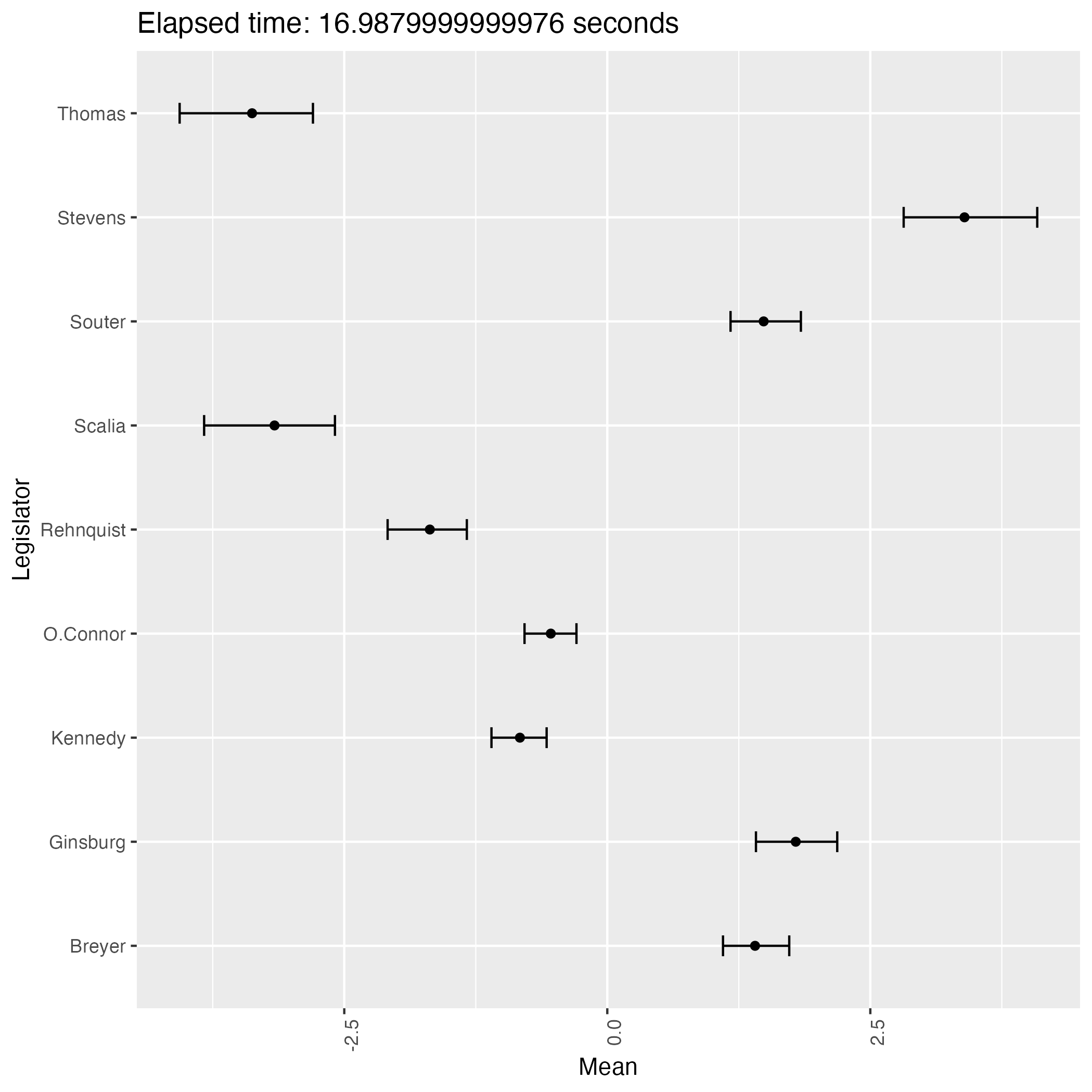
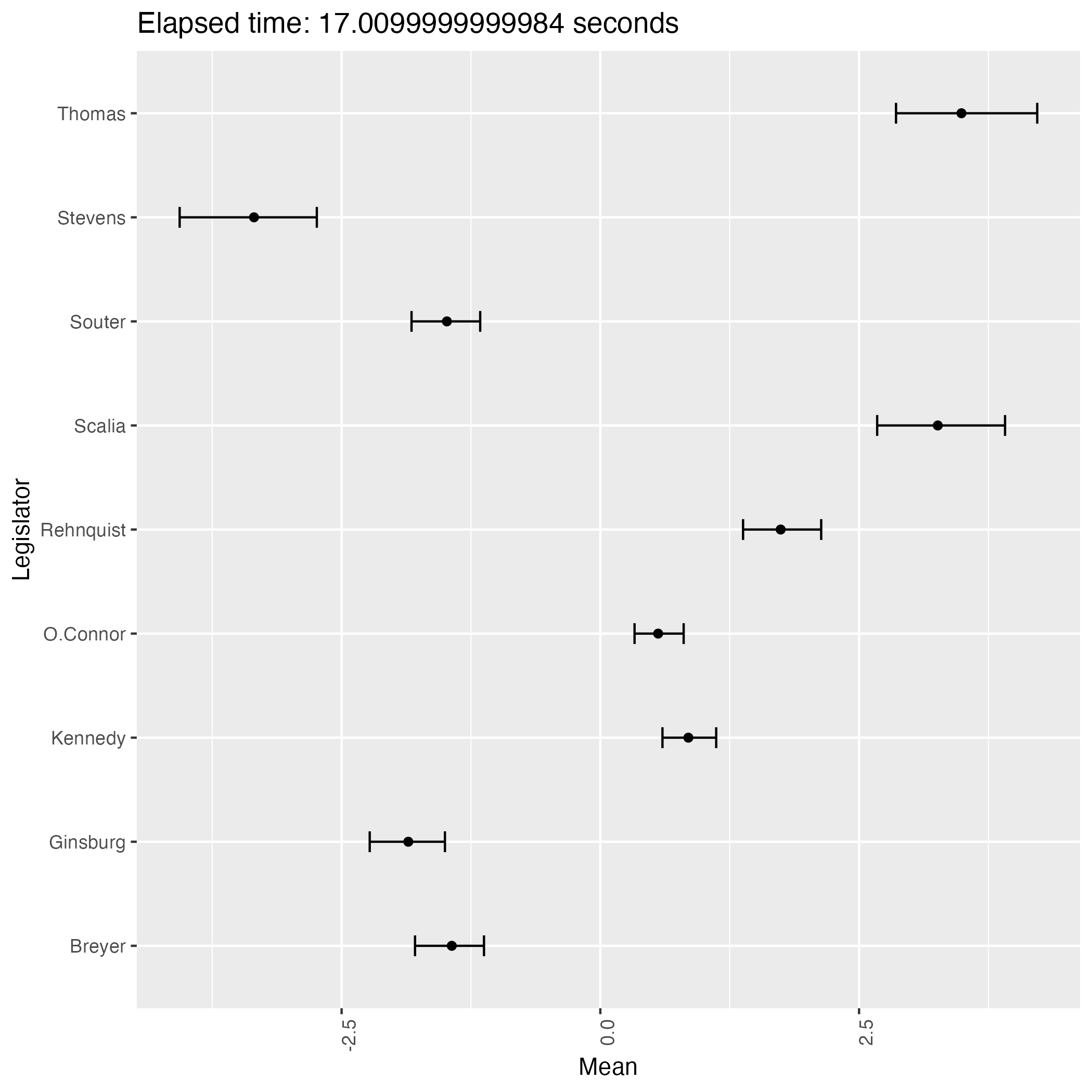
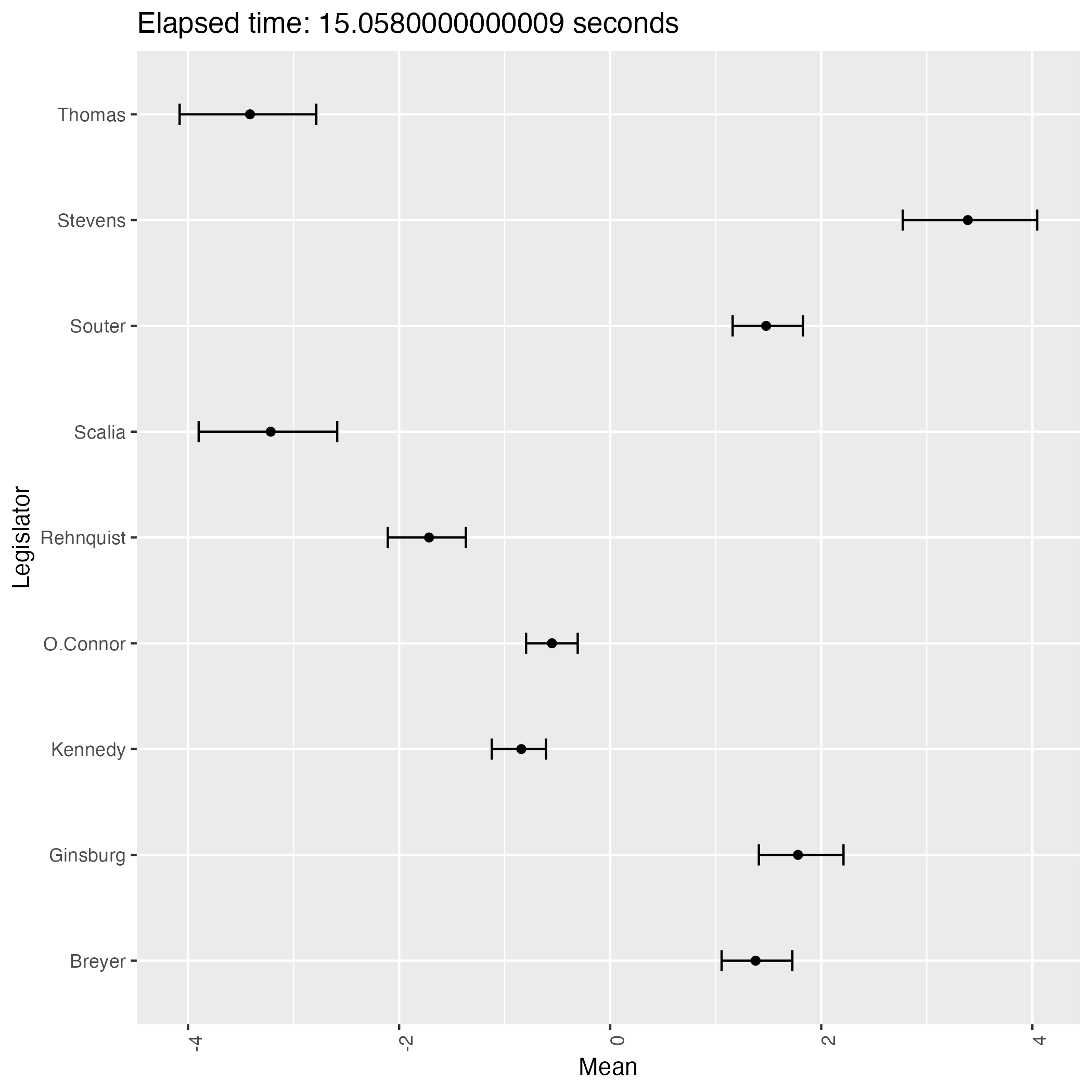
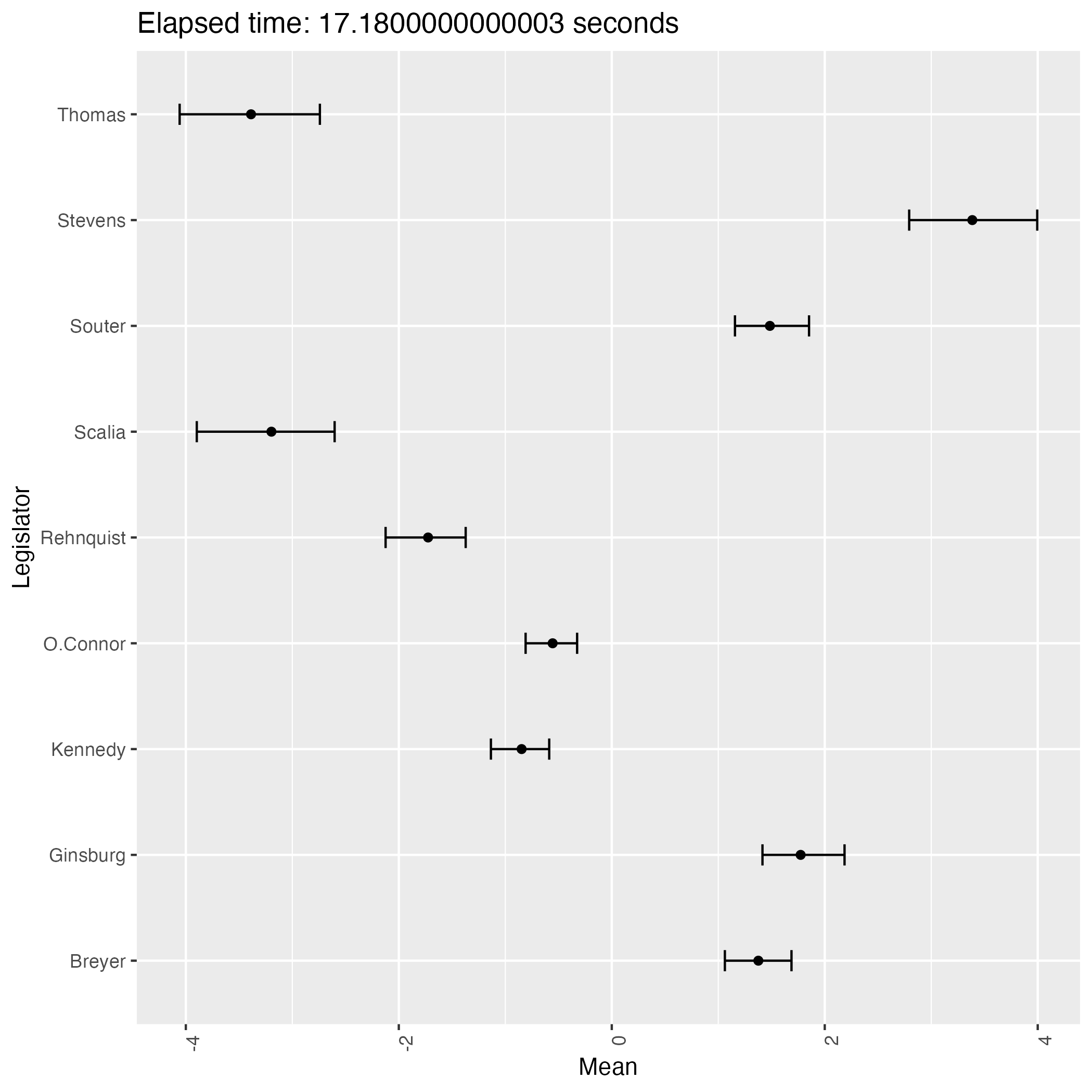
The following plots are some (first 9) of the results from the experiment.

Elapsed time: 16.99 seconds

Elapsed time: 17.01 seconds

Elapsed time: 16.30 seconds

Elapsed time: 15.00 seconds

Elapsed time: 14.98 seconds

Elapsed time: 15.06 seconds

Elapsed time: 16.42 seconds

Elapsed time: 16.57 seconds

Elapsed time: 17.18 seconds

We see that the result has two patterns and they are in symmetry with each other.

This phenomenon proves that the posterior distribution of the ideal points is bimodal, indicating the weak identifiability of the model.

3 Conclusion

(Bafumi et al., 2005)’s hierarchical resolution of the identifiability problem by the covariate $Z_i$ will fail if the covariate $Z_i$ is not informative enough.

In that case, the posterior distribution of the ideal points will be bimodal.

References

Bafumi, J., Gelman, A., Park, D. K., and Kaplan, N. (2005). Practical Issues in Implementing and Understanding Bayesian Ideal Point Estimation. Political Analysis, 13(2), 171–187.

Martin, A. D., Quinn, K. M., and Park, J. H. (2011). MCMCpack: Markov chain Monte Carlo in R. Journal of Statistical Software, 42(9), 1–21.

Copyright

Copyright Hirofumi Shiba 2024. All Rights Reserved