或る区分確定的マルコフ過程のスケーリング極限

1 背景：PDMP とその特殊性

モンテカルロ法に用いられる PDMP の例：Forward Event-Chain Monte Carlo

A Blog Entry on Bayesian Computation by an Applied Mathematician

$$

$$

1.1 モンテカルロ法小史

酔歩
（1953〜）

拡散過程
（1978〜）

PDMP
（2008〜）

1.2 Piecewise Deterministic Markov Process

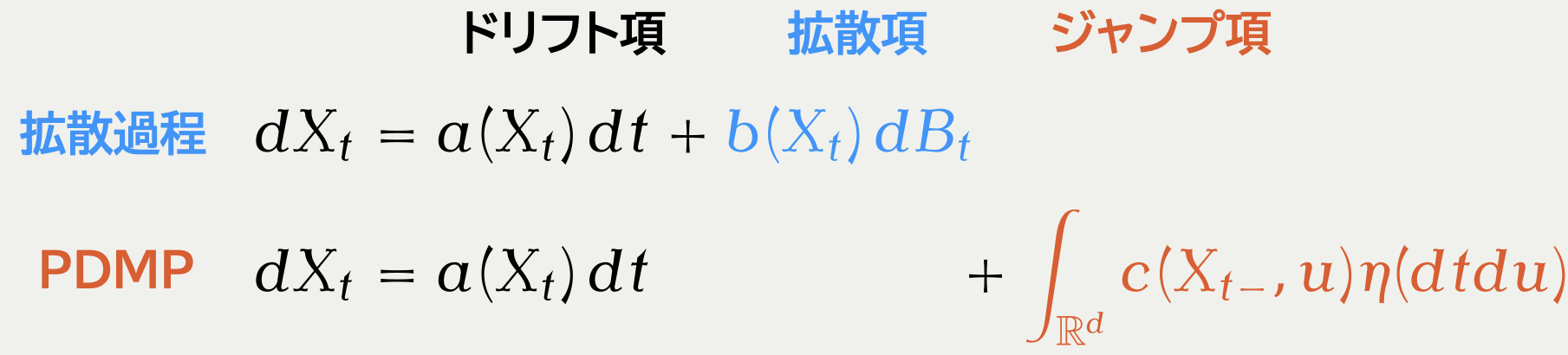
直感：SDE より ODE の離散化の方が「扱いやすい」

Langevin Diffusion

Randomized Hamiltonian Monte Carlo

1.3 HMC v. PDMP：高次元ではほぼ同じ．離散化が違うのみ

PDMP サンプラーは ODE Solver なしで Hamiltonian flow を近似できる

RHMC (d=2)

symplectic integrator で離散化

O(d^{1.25}) の計算複雑性

BPS with Gaussian speed (d=10^3)

大量の Poisson 点測度 で近似

通常時は O(d^{1.5}) の計算複雑性

1.4 PDMP は killer application での爆発力がすごい

横軸：時間，縦軸：推定量．(Bouchard-Côté et al., 2018)
スパースな相互作用を持つマルコフ確率場モデル（d=10）

局所実装 O(d^1)

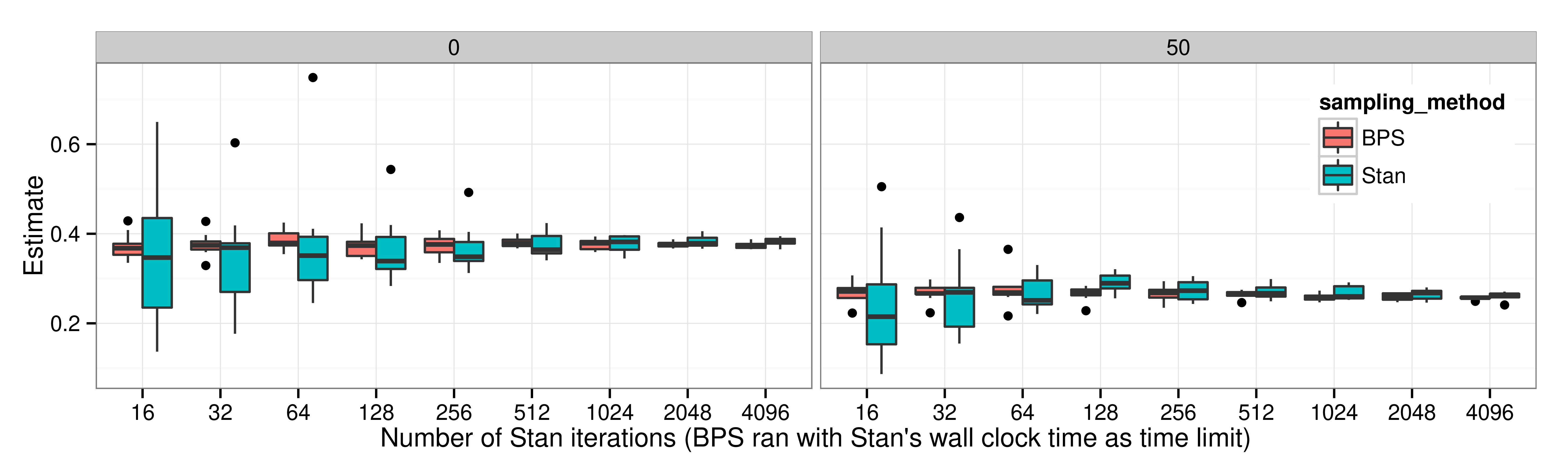
BPS で，sparsity を利用した実装をすると，HMC よりも「推定量の分散／時」が良い．

(Bierkens et al., 2019)

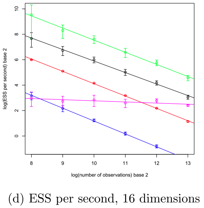
Stochastic Gradient O(n^0)

横軸：観測数 n，縦軸：有効サンプルサイズ．
ロジスティック回帰（d=16）．
Zig-Zag で，control variate を用いると，データサイズ n に対して O(1) の性能
n\to\infty の極限で Langevin を越す．

2 等速直線ダイナミクス
でどこまで行けるか？

HMC は Metropolis–Hastings 界のトップ．PDMP のトップは？

• スケーリング解析の導入＋既存研究 (2.1 – 2.5)
• 今回の研究成果 (2.6 – 2.12)

2.1 BPS の大域的リフレッシュパラメータ \rho

2.2 BPS \textcolor{#0096FF}{\{X_t\}} のスケーリング解析

定常分布 X_0\sim\pi から実行したときの低次元射影 \textcolor{#0096FF}{Y_t^{(d)}}:=\frac{U(\textcolor{#0096FF}{X_{d^\gamma t}})-\operatorname{E}_\pi[U(\textcolor{#0096FF}{X_{d^\gamma t}})]}{\sqrt{\operatorname{Var}_\pi[U(\textcolor{#0096FF}{X_{d^\gamma t}})]}},\quad U:\mathbb{R}^d\to\mathbb{R}\text{: 射影},\;\textcolor{#0096FF}{\gamma}>0 の，d\to\infty の極限での挙動を解析する．

Tip定義（最適スケーリング \gamma）

\textcolor{#0096FF}{Y_t^{(d)}} がある \gamma>0 について，d\to\infty の極限で拡散過程に収束するとき，この \gamma を 最適スケーリング という．

Important射影 U の例

• 有限次元周辺過程：U(x)=x_1
• 負の対数密度：U(x)=-\log\pi(x)

Important\gamma の例 （U(x)=x_1 のとき）

• 酔歩 MH は \gamma=1
• Langevin は \gamma=1/3

2.3 BPS の拡散スケーリング極限（\gamma=1）

\textcolor{#0096FF}{Y_t^{(d)}} を U(x)=-\log\pi(x) について，d=10^2,10^3,10^4 でプロットしてみる：

2.4 先行研究：Zig-Zag v. BPS (Bierkens et al., 2022)

あるカーネル L を持つ Gauss 過程

L(s,t)=2-\int^t_s\int^t_sK(u,v)\,dudv

K は動径運動量 R のカーネル K(s,t)=\operatorname{E}[R_sR_t]

Ornstein-Uhlenbeck 過程

dY_t=-\frac{\sigma^2(\rho)}{4}Y_t\,dt+\sigma(\rho)\,dB_t \sigma^2(\rho)=8\int^\infty_0e^{-\rho s}K(s,0)\,ds

2.5 拡散係数 \sigma の近似 → 漸近最適なハイパラ選択基準

2.6 FECMC という新星：\rho の排除

2.7 効率性比較：Zig-Zag v. BPS v. FECMC

100 次元 Gauss の U(x)=\|x\|^2 推定における有効サンプルサイズ (ESS)．1000 回実行して推定．

2.8 主貢献1：FECMC のスケーリング極限は BPS と同じ形

dY_t^{\textcolor{#0096FF}{\text{B}}}=-\frac{\sigma^2_{\textcolor{#0096FF}{\text{B}}}(\rho)}{4}Y_t^{\textcolor{#0096FF}{\text{B}}}\,dt+\sigma_{\textcolor{#0096FF}{\text{B}}}(\rho)\,dB_t \sigma^2_{\textcolor{#0096FF}{\text{B}}}(\rho)=8\int^\infty_0e^{-\rho s}\operatorname{E}[R_0^{\textcolor{#0096FF}{\text{B}}}R_s^{\textcolor{#0096FF}{\text{B}}}]\,ds

dY_t^{\textcolor{#E95420}{\text{F}}}=-\frac{\sigma^2_{\textcolor{#E95420}{\text{F}}}(\rho)}{4}Y_t^{\textcolor{#E95420}{\text{F}}}\,dt+\sigma_{\textcolor{#E95420}{\text{F}}}(\rho)\,dB_t \sigma^2_{\textcolor{#E95420}{\text{F}}}(\rho)=8\int^\infty_0e^{-\rho s}\operatorname{E}[R_0^{\textcolor{#E95420}{\text{F}}}R_s^{\textcolor{#E95420}{\text{F}}}]\,ds

2.9 主貢献2：拡散係数の解析的表示

\begin{align*} \sigma^2_{\textcolor{#E95420}{\text{FECMC}}}(\rho)&=\sqrt{\frac{32}{\pi}}\biggr(1-\frac{\left(\rho^2-\rho\sqrt{\frac{\pi}{2}}+\Omega(\rho)\right)^2}{\rho^4\Omega(\rho)(2-\Omega(\rho))}\biggl)\\ \sigma^2_{\textcolor{#0096FF}{\text{BPS}}}(\rho)&=\frac{8}{\rho^4}\left(\rho^3-\rho^2\sqrt{\frac{8}{\pi}}+\rho-\sqrt{\frac{8}{\pi}}\frac{\left((1+\rho^2)\Omega(\rho)-\rho^2\right)^2}{\Omega(2\rho)}\right)\\ \Omega(\rho)&\coloneqq\sqrt{\frac{\pi}{2}}\rho\operatorname{erfcx}\left(\frac{\rho}{\sqrt{2}}\right)=\rho e^{\frac{\rho^2}{2}}\int^\infty_\rho e^{-\frac{t^2}{2}}\,\mathrm{d}t \end{align*}

\begin{align*} \underbrace{\frac{\sigma^2(0)}{4}=2\int^\infty_0\operatorname{E}[R_0R_t]\,dt}_{\text{Green--Kubo 公式}}=\operatorname{E}\biggl[R_0\underbrace{\int^\infty_0\operatorname{E}[R_t|R_0]\,dt}_{=:f(R_0)}\biggr]=\operatorname{E}[R_0f(R_0)] \end{align*} この関数 f は，動径運動量 R の生成作用素 L に関して次を満たす： -Lf(x)=x\quad\text{（Poisson 方程式）}

2.10 拡散係数の比較 FECMC v. BPS

2.11 拡散係数 \sigma ≒ モンテカルロ漸近分散 ≒ ESS

Tip系（拡散係数 \sigma が大きいと ESS も大きい）

U を長さ T の軌跡で推定する際の有効サンプルサイズ (ESS) は \operatorname{ESS}(U)=\frac{T\sigma^2}{8}.

【説明】 モンテカルロ推定量（＝PDMP \textcolor{#0096FF}{\{X_t\}} の時間平均） \widehat{h}_T:=\frac{1}{T}\int^T_0U(\textcolor{#0096FF}{X_s})\,ds の漸近分散比は，高次元極限では次で与えられる： \lim_{T\to\infty}\lim_{d\to\infty}T\frac{\operatorname{Var}[\widehat{h}_{\textcolor{#E95420}{d}T}]}{\operatorname{Var}_\pi[U(X)]}=\frac{8}{\sigma^2}\approx2.50\cdots. この逆数が単位時間あたりの有効サンプルサイズである．

2.12 実験との整合：FECMC v. BPS

3 応用：PDMP の収束判定

実際の分布 \pi では \sigma^2 の値はわからない．これを推定するのが収束判定．

PDMP には補助変数 \textcolor{#E95420}{\{V_t\}} があり，これを利用することでモンテカルロ漸近分散の推定量の分散を改善することができる．

• 理論（スライド 3.1 & 3.2）
• 実験（スライド 3.3 & 3.4）

3.1 漸近分散推定における fast proxy

推定対象 U(x)=-\log\pi(x) の代わりに，その時間微分 \textcolor{#E95420}{g(x,\dot{x})}:=\dot{U} を考える \text{例：}\quad U(x)=\frac{\|x\|^2}{2}\quad\text{のときは}\quad \textcolor{#E95420}{g(x,v)}=\langle x,v\rangle.

２種類のモンテカルロ推定量を考える：

\widehat{h}_T:=\frac{1}{T}\int^T_0U(X_s)\,ds,\quad \textcolor{#E95420}{\widehat{g}_T}:=\frac{1}{T}\int^T_0\textcolor{#E95420}{g(X_t,V_t)}\,dt.

Tip系（モンテカルロ漸近分散は逆にして２倍の値になる）

\lim_{T\to\infty}\lim_{d\to\infty}T\frac{\operatorname{Var}[\widehat{h}_{\textcolor{#E95420}{d}T}]}{\operatorname{Var}_\pi[U(X)]}=\frac{8}{\sigma^2},\quad \lim_{T\to\infty}\lim_{d\to\infty}T\frac{\operatorname{Var}[\textcolor{#E95420}{\widehat{g}_{T}}]}{\operatorname{Var}_{\pi\otimes\mu}[\textcolor{#E95420}{g(X,V)}]}=\frac{\sigma^2}{4}.

→ \textcolor{#E95420}{d} が大きいほど，\sigma^2 の値を知るのに，\textcolor{#E95420}{\widehat{g}_T} を使った方が有利？

3.2 漸近分散推定量の例 Batch Means Estimator

Tip系（\hat{h} と \textcolor{#E95420}{\hat{g}} のモンテカルロ漸近分散）

\lim_{T\to\infty}\lim_{d\to\infty}T\frac{\operatorname{Var}[\widehat{h}_{\textcolor{#E95420}{d}T}]}{\operatorname{Var}_\pi[U(X)]}=\frac{8}{\sigma^2},\quad \lim_{T\to\infty}\lim_{d\to\infty}T\frac{\operatorname{Var}[\textcolor{#E95420}{\widehat{g}_{T}}]}{\operatorname{Var}_{\pi\otimes\mu}[\textcolor{#E95420}{g(X,V)}]}=\frac{\sigma^2}{4}.

batch size b>0 を設定し，その小区間平均 h_i:=\frac{1}{b}\int^{ib}_{(i-1)b}U(X_t)\,dt の全体 h_1,h_2,\cdots,h_B の不偏分散の b 倍を batch means 推定量という： \textcolor{#0096FF}{\frac{b}{B-1}\sum_{i=1}^B(h_i-\overline{h})}\xrightarrow[\text{適切な極限}]{T\to\infty}\lim_{d\to\infty}\lim_{T\to\infty}T\frac{\operatorname{Var}[\widehat{h}_{\textcolor{#E95420}{d}T}]}{\operatorname{Var}_\pi[U(X)]}=\frac{8}{\sigma^2}\;\;(\textbf{一致性}). MSE の意味で最適な b>0 が判っている (Liu et al., 2022)．

3.3 実験結果：既存手法 v. 提案手法

3.4 非等方的 Gauss：既存手法 v. 提案手法

4 引用文献

Bierkens, J., Fearnhead, P., and Roberts, G. (2019). The Zig-Zag Process and Super-Efficient Sampling for Bayesian Analysis of Big Data. The Annals of Statistics, 47(3), 1288–1320.

Bierkens, J., Kamatani, K., and Roberts, G. O. (2022). High-Dimensional Scaling Limits of Piecewise Deterministic Sampling Algorithms. The Annals of Applied Probability, 32(5), 3361–3407.

Bouchard-Côté, A., Vollmer, S. J., and Doucet, A. (2018). The Bouncy Particle Sampler: A Nonreversible Rejection-Free Markov Chain Monte Carlo Method. Journal of the American Statistical Association, 113(522), 855–867.

Liu, Y., Vats, D., and Flegal, J. M. (2022). Batch size selection for variance estimators in MCMC. Methodology and Computing in Applied Probability, 24(1), 65–93.