R によるベイズ混合モデリング入門

brms を用いた混合効果モデリング入門

Bayesian
MCMC
R
Stan
Statistics
Author

司馬博文

Published

5/12/2024

Modified

9/12/2024

概要

brms はベイズ階層モデリングを,確率的プログラミング言語 Stan をエンジンとして行うための R パッケージである.本稿では,brms の基本的な使い方と,その実装を紹介する.

また,ランダム効果モデルとは何であるか,固定効果モデル・混合効果モデル・一般化推定方程式などとの違いをレビューする.ランダム効果の追加は縮小推定などの自動的な正則化を可能とする美点がある一方で,係数の不偏推定やロバスト推定に拘る場合はこれを避ける判断もあり得る.

brms: Bayesian Regression Models using ‘Stan’ リンク集

ダウンロードは:1

install.packages("brms")

1 例で学ぶ brms の使い方

1.1 カウントデータのモデリング

Documentation で紹介されている,Epilepsy Seizures Data (Leppik et al., 1987)(Thall and Vail, 1990) を用いた を実行してみる:

library(brms)
fit1 <- brm(count ~ zAge + zBase * Trt + (1|patient),
            data = epilepsy, family = poisson())

てんかん (epilepsy) 患者の発作回数countを被説明変数とし,処置の効果を表す説明変数Trtと患者毎のランダムな切片項(1|patient),及びzAge,zBaseへの依存構造を調べたい.

被説明変数countは離散変数であり,Poisson 分布に従うと仮定する.

説明変数
  • zAge:標準化された年齢
  • zBase:ベースの発作回数
  • Trt:治療の有無を表す2値変数
  • (1|patient):患者ごとに異なるとした切片項

zBase * Trtという記法は,この2つの交互作用もモデルに含めることを意味する.

データの詳細

epilepsyは59 人の患者に関して,4回の入院時の発作回数を記録した,全 236 データからなる.patientが患者を識別する ID であり,(1|patient)は患者ごとのランダム効果ということになる.

従って本モデルはzAge, zBase, Trt, Trt*zBaseという固定効果,(1|patient)というランダム効果を取り入れた(一般化線型)混合効果モデル ということになり,回帰式は次の通りである: \[ y_{it} = \beta_1 \cdot\texttt{zAge}_i+ \beta_2 \cdot \texttt{zBase}_i + \beta_3 \cdot \texttt{Trt}_i \] \[ + \beta_4 \cdot (\texttt{zBase}_i \cdot \texttt{Trt}_i) + \alpha_i +\epsilon_{it}. \] ただし,\(\texttt{count}_{it}\) の Poisson 母数を \(\lambda_{it}\) として,\(y_{it}:=\log(\lambda_{it})\) とした.

解析意図としては,ベースの発作回数が高いほど,治療効果が高い/低いのではないか?という仮説を検証する,zBase*Trtを曝露因子としたモデルである.

epilepsy
    Age Base Trt patient visit count obs        zAge        zBase
1    31   11   0       1     1     5   1  0.42499501 -0.757172825
2    30   11   0       2     1     3   2  0.26528351 -0.757172825
3    25    6   0       3     1     2   3 -0.53327400 -0.944403322
4    36    8   0       4     1     4   4  1.22355252 -0.869511123
5    22   66   0       5     1     7   5 -1.01240850  1.302362646
6    29   27   0       6     1     5   6  0.10557201 -0.158035233
7    31   12   0       7     1     6   7  0.42499501 -0.719726725
8    42   52   0       8     1    40   8  2.18182153  0.778117253
9    37   23   0       9     1     5   9  1.38326402 -0.307819631
10   28   10   0      10     1    14  10 -0.05413949 -0.794618924
11   36   52   0      11     1    26  11  1.22355252  0.778117253
12   24   33   0      12     1    12  12 -0.69298550  0.066641363
13   23   18   0      13     1     4  13 -0.85269700 -0.495050128
14   36   42   0      14     1     7  14  1.22355252  0.403656259
15   26   87   0      15     1    16  15 -0.37356249  2.088730734
16   26   50   0      16     1    11  16 -0.37356249  0.703225054
17   28   18   0      17     1     0  17 -0.05413949 -0.495050128
18   31  111   0      18     1    37  18  0.42499501  2.987437121
19   32   18   0      19     1     3  19  0.58470651 -0.495050128
20   21   20   0      20     1     3  20 -1.17212000 -0.420157930
21   29   12   0      21     1     3  21  0.10557201 -0.719726725
22   21    9   0      22     1     3  22 -1.17212000 -0.832065024
23   32   17   0      23     1     2  23  0.58470651 -0.532496228
24   25   28   0      24     1     8  24 -0.53327400 -0.120589134
25   30   55   0      25     1    18  25  0.26528351  0.890455552
26   40    9   0      26     1     2  26  1.86239852 -0.832065024
27   19   10   0      27     1     3  27 -1.49154300 -0.794618924
28   22   47   0      28     1    13  28 -1.01240850  0.590886756
29   18   76   1      29     1    11  29 -1.65125450  1.676823640
30   32   38   1      30     1     8  30  0.58470651  0.253871861
31   20   19   1      31     1     0  31 -1.33183150 -0.457604029
32   30   10   1      32     1     3  32  0.26528351 -0.794618924
33   18   19   1      33     1     2  33 -1.65125450 -0.457604029
34   24   24   1      34     1     4  34 -0.69298550 -0.270373532
35   30   31   1      35     1    22  35  0.26528351 -0.008250835
36   35   14   1      36     1     5  36  1.06384102 -0.644834526
37   27   11   1      37     1     2  37 -0.21385099 -0.757172825
38   20   67   1      38     1     3  38 -1.33183150  1.339808745
39   22   41   1      39     1     4  39 -1.01240850  0.366210159
40   28    7   1      40     1     2  40 -0.05413949 -0.906957223
41   23   22   1      41     1     0  41 -0.85269700 -0.345265731
42   40   13   1      42     1     5  42  1.86239852 -0.682280626
43   33   46   1      43     1    11  43  0.74441801  0.553440656
44   21   36   1      44     1    10  44 -1.17212000  0.178979662
45   35   38   1      45     1    19  45  1.06384102  0.253871861
46   25    7   1      46     1     1  46 -0.53327400 -0.906957223
47   26   36   1      47     1     6  47 -0.37356249  0.178979662
48   25   11   1      48     1     2  48 -0.53327400 -0.757172825
49   22  151   1      49     1   102  49 -1.01240850  4.485281100
50   32   22   1      50     1     4  50  0.58470651 -0.345265731
51   25   41   1      51     1     8  51 -0.53327400  0.366210159
52   35   32   1      52     1     1  52  1.06384102  0.029195264
53   21   56   1      53     1    18  53 -1.17212000  0.927901651
54   41   24   1      54     1     6  54  2.02211002 -0.270373532
55   32   16   1      55     1     3  55  0.58470651 -0.569942327
56   26   22   1      56     1     1  56 -0.37356249 -0.345265731
57   21   25   1      57     1     2  57 -1.17212000 -0.232927432
58   36   13   1      58     1     0  58  1.22355252 -0.682280626
59   37   12   1      59     1     1  59  1.38326402 -0.719726725
60   31   11   0       1     2     3  60  0.42499501 -0.757172825
61   30   11   0       2     2     5  61  0.26528351 -0.757172825
62   25    6   0       3     2     4  62 -0.53327400 -0.944403322
63   36    8   0       4     2     4  63  1.22355252 -0.869511123
64   22   66   0       5     2    18  64 -1.01240850  1.302362646
65   29   27   0       6     2     2  65  0.10557201 -0.158035233
66   31   12   0       7     2     4  66  0.42499501 -0.719726725
67   42   52   0       8     2    20  67  2.18182153  0.778117253
68   37   23   0       9     2     6  68  1.38326402 -0.307819631
69   28   10   0      10     2    13  69 -0.05413949 -0.794618924
70   36   52   0      11     2    12  70  1.22355252  0.778117253
71   24   33   0      12     2     6  71 -0.69298550  0.066641363
72   23   18   0      13     2     4  72 -0.85269700 -0.495050128
73   36   42   0      14     2     9  73  1.22355252  0.403656259
74   26   87   0      15     2    24  74 -0.37356249  2.088730734
75   26   50   0      16     2     0  75 -0.37356249  0.703225054
76   28   18   0      17     2     0  76 -0.05413949 -0.495050128
77   31  111   0      18     2    29  77  0.42499501  2.987437121
78   32   18   0      19     2     5  78  0.58470651 -0.495050128
79   21   20   0      20     2     0  79 -1.17212000 -0.420157930
80   29   12   0      21     2     4  80  0.10557201 -0.719726725
81   21    9   0      22     2     4  81 -1.17212000 -0.832065024
82   32   17   0      23     2     3  82  0.58470651 -0.532496228
83   25   28   0      24     2    12  83 -0.53327400 -0.120589134
84   30   55   0      25     2    24  84  0.26528351  0.890455552
85   40    9   0      26     2     1  85  1.86239852 -0.832065024
86   19   10   0      27     2     1  86 -1.49154300 -0.794618924
87   22   47   0      28     2    15  87 -1.01240850  0.590886756
88   18   76   1      29     2    14  88 -1.65125450  1.676823640
89   32   38   1      30     2     7  89  0.58470651  0.253871861
90   20   19   1      31     2     4  90 -1.33183150 -0.457604029
91   30   10   1      32     2     6  91  0.26528351 -0.794618924
92   18   19   1      33     2     6  92 -1.65125450 -0.457604029
93   24   24   1      34     2     3  93 -0.69298550 -0.270373532
94   30   31   1      35     2    17  94  0.26528351 -0.008250835
95   35   14   1      36     2     4  95  1.06384102 -0.644834526
96   27   11   1      37     2     4  96 -0.21385099 -0.757172825
97   20   67   1      38     2     7  97 -1.33183150  1.339808745
98   22   41   1      39     2    18  98 -1.01240850  0.366210159
99   28    7   1      40     2     1  99 -0.05413949 -0.906957223
100  23   22   1      41     2     2 100 -0.85269700 -0.345265731
101  40   13   1      42     2     4 101  1.86239852 -0.682280626
102  33   46   1      43     2    14 102  0.74441801  0.553440656
103  21   36   1      44     2     5 103 -1.17212000  0.178979662
104  35   38   1      45     2     7 104  1.06384102  0.253871861
105  25    7   1      46     2     1 105 -0.53327400 -0.906957223
106  26   36   1      47     2    10 106 -0.37356249  0.178979662
107  25   11   1      48     2     1 107 -0.53327400 -0.757172825
108  22  151   1      49     2    65 108 -1.01240850  4.485281100
109  32   22   1      50     2     3 109  0.58470651 -0.345265731
110  25   41   1      51     2     6 110 -0.53327400  0.366210159
111  35   32   1      52     2     3 111  1.06384102  0.029195264
112  21   56   1      53     2    11 112 -1.17212000  0.927901651
113  41   24   1      54     2     3 113  2.02211002 -0.270373532
114  32   16   1      55     2     5 114  0.58470651 -0.569942327
115  26   22   1      56     2    23 115 -0.37356249 -0.345265731
116  21   25   1      57     2     3 116 -1.17212000 -0.232927432
117  36   13   1      58     2     0 117  1.22355252 -0.682280626
118  37   12   1      59     2     4 118  1.38326402 -0.719726725
119  31   11   0       1     3     3 119  0.42499501 -0.757172825
120  30   11   0       2     3     3 120  0.26528351 -0.757172825
121  25    6   0       3     3     0 121 -0.53327400 -0.944403322
122  36    8   0       4     3     1 122  1.22355252 -0.869511123
123  22   66   0       5     3     9 123 -1.01240850  1.302362646
124  29   27   0       6     3     8 124  0.10557201 -0.158035233
125  31   12   0       7     3     0 125  0.42499501 -0.719726725
126  42   52   0       8     3    21 126  2.18182153  0.778117253
127  37   23   0       9     3     6 127  1.38326402 -0.307819631
128  28   10   0      10     3     6 128 -0.05413949 -0.794618924
129  36   52   0      11     3     6 129  1.22355252  0.778117253
130  24   33   0      12     3     8 130 -0.69298550  0.066641363
131  23   18   0      13     3     6 131 -0.85269700 -0.495050128
132  36   42   0      14     3    12 132  1.22355252  0.403656259
133  26   87   0      15     3    10 133 -0.37356249  2.088730734
134  26   50   0      16     3     0 134 -0.37356249  0.703225054
135  28   18   0      17     3     3 135 -0.05413949 -0.495050128
136  31  111   0      18     3    28 136  0.42499501  2.987437121
137  32   18   0      19     3     2 137  0.58470651 -0.495050128
138  21   20   0      20     3     6 138 -1.17212000 -0.420157930
139  29   12   0      21     3     3 139  0.10557201 -0.719726725
140  21    9   0      22     3     3 140 -1.17212000 -0.832065024
141  32   17   0      23     3     3 141  0.58470651 -0.532496228
142  25   28   0      24     3     2 142 -0.53327400 -0.120589134
143  30   55   0      25     3    76 143  0.26528351  0.890455552
144  40    9   0      26     3     2 144  1.86239852 -0.832065024
145  19   10   0      27     3     4 145 -1.49154300 -0.794618924
146  22   47   0      28     3    13 146 -1.01240850  0.590886756
147  18   76   1      29     3     9 147 -1.65125450  1.676823640
148  32   38   1      30     3     9 148  0.58470651  0.253871861
149  20   19   1      31     3     3 149 -1.33183150 -0.457604029
150  30   10   1      32     3     1 150  0.26528351 -0.794618924
151  18   19   1      33     3     7 151 -1.65125450 -0.457604029
152  24   24   1      34     3     1 152 -0.69298550 -0.270373532
153  30   31   1      35     3    19 153  0.26528351 -0.008250835
154  35   14   1      36     3     7 154  1.06384102 -0.644834526
155  27   11   1      37     3     0 155 -0.21385099 -0.757172825
156  20   67   1      38     3     7 156 -1.33183150  1.339808745
157  22   41   1      39     3     2 157 -1.01240850  0.366210159
158  28    7   1      40     3     1 158 -0.05413949 -0.906957223
159  23   22   1      41     3     4 159 -0.85269700 -0.345265731
160  40   13   1      42     3     0 160  1.86239852 -0.682280626
161  33   46   1      43     3    25 161  0.74441801  0.553440656
162  21   36   1      44     3     3 162 -1.17212000  0.178979662
163  35   38   1      45     3     6 163  1.06384102  0.253871861
164  25    7   1      46     3     2 164 -0.53327400 -0.906957223
165  26   36   1      47     3     8 165 -0.37356249  0.178979662
166  25   11   1      48     3     0 166 -0.53327400 -0.757172825
167  22  151   1      49     3    72 167 -1.01240850  4.485281100
168  32   22   1      50     3     2 168  0.58470651 -0.345265731
169  25   41   1      51     3     5 169 -0.53327400  0.366210159
170  35   32   1      52     3     1 170  1.06384102  0.029195264
171  21   56   1      53     3    28 171 -1.17212000  0.927901651
172  41   24   1      54     3     4 172  2.02211002 -0.270373532
173  32   16   1      55     3     4 173  0.58470651 -0.569942327
174  26   22   1      56     3    19 174 -0.37356249 -0.345265731
175  21   25   1      57     3     0 175 -1.17212000 -0.232927432
176  36   13   1      58     3     0 176  1.22355252 -0.682280626
177  37   12   1      59     3     3 177  1.38326402 -0.719726725
178  31   11   0       1     4     3 178  0.42499501 -0.757172825
179  30   11   0       2     4     3 179  0.26528351 -0.757172825
180  25    6   0       3     4     5 180 -0.53327400 -0.944403322
181  36    8   0       4     4     4 181  1.22355252 -0.869511123
182  22   66   0       5     4    21 182 -1.01240850  1.302362646
183  29   27   0       6     4     7 183  0.10557201 -0.158035233
184  31   12   0       7     4     2 184  0.42499501 -0.719726725
185  42   52   0       8     4    12 185  2.18182153  0.778117253
186  37   23   0       9     4     5 186  1.38326402 -0.307819631
187  28   10   0      10     4     0 187 -0.05413949 -0.794618924
188  36   52   0      11     4    22 188  1.22355252  0.778117253
189  24   33   0      12     4     4 189 -0.69298550  0.066641363
190  23   18   0      13     4     2 190 -0.85269700 -0.495050128
191  36   42   0      14     4    14 191  1.22355252  0.403656259
192  26   87   0      15     4     9 192 -0.37356249  2.088730734
193  26   50   0      16     4     5 193 -0.37356249  0.703225054
194  28   18   0      17     4     3 194 -0.05413949 -0.495050128
195  31  111   0      18     4    29 195  0.42499501  2.987437121
196  32   18   0      19     4     5 196  0.58470651 -0.495050128
197  21   20   0      20     4     7 197 -1.17212000 -0.420157930
198  29   12   0      21     4     4 198  0.10557201 -0.719726725
199  21    9   0      22     4     4 199 -1.17212000 -0.832065024
200  32   17   0      23     4     5 200  0.58470651 -0.532496228
201  25   28   0      24     4     8 201 -0.53327400 -0.120589134
202  30   55   0      25     4    25 202  0.26528351  0.890455552
203  40    9   0      26     4     1 203  1.86239852 -0.832065024
204  19   10   0      27     4     2 204 -1.49154300 -0.794618924
205  22   47   0      28     4    12 205 -1.01240850  0.590886756
206  18   76   1      29     4     8 206 -1.65125450  1.676823640
207  32   38   1      30     4     4 207  0.58470651  0.253871861
208  20   19   1      31     4     0 208 -1.33183150 -0.457604029
209  30   10   1      32     4     3 209  0.26528351 -0.794618924
210  18   19   1      33     4     4 210 -1.65125450 -0.457604029
211  24   24   1      34     4     3 211 -0.69298550 -0.270373532
212  30   31   1      35     4    16 212  0.26528351 -0.008250835
213  35   14   1      36     4     4 213  1.06384102 -0.644834526
214  27   11   1      37     4     4 214 -0.21385099 -0.757172825
215  20   67   1      38     4     7 215 -1.33183150  1.339808745
216  22   41   1      39     4     5 216 -1.01240850  0.366210159
217  28    7   1      40     4     0 217 -0.05413949 -0.906957223
218  23   22   1      41     4     0 218 -0.85269700 -0.345265731
219  40   13   1      42     4     3 219  1.86239852 -0.682280626
220  33   46   1      43     4    15 220  0.74441801  0.553440656
221  21   36   1      44     4     8 221 -1.17212000  0.178979662
222  35   38   1      45     4     7 222  1.06384102  0.253871861
223  25    7   1      46     4     3 223 -0.53327400 -0.906957223
224  26   36   1      47     4     8 224 -0.37356249  0.178979662
225  25   11   1      48     4     0 225 -0.53327400 -0.757172825
226  22  151   1      49     4    63 226 -1.01240850  4.485281100
227  32   22   1      50     4     4 227  0.58470651 -0.345265731
228  25   41   1      51     4     7 228 -0.53327400  0.366210159
229  35   32   1      52     4     5 229  1.06384102  0.029195264
230  21   56   1      53     4    13 230 -1.17212000  0.927901651
231  41   24   1      54     4     0 231  2.02211002 -0.270373532
232  32   16   1      55     4     3 232  0.58470651 -0.569942327
233  26   22   1      56     4     8 233 -0.37356249 -0.345265731
234  21   25   1      57     4     1 234 -1.17212000 -0.232927432
235  36   13   1      58     4     0 235  1.22355252 -0.682280626
236  37   12   1      59     4     2 236  1.38326402 -0.719726725

1.2 モデルの推定とプロット

library(brms)
fit1 <- brm(count ~ zAge + zBase * Trt + (1|patient),
            data = epilepsy, family = poisson())
Compiling Stan program...
Start sampling

SAMPLING FOR MODEL 'anon_model' NOW (CHAIN 1).
Chain 1: 
Chain 1: Gradient evaluation took 5.2e-05 seconds
Chain 1: 1000 transitions using 10 leapfrog steps per transition would take 0.52 seconds.
Chain 1: Adjust your expectations accordingly!
Chain 1: 
Chain 1: 
Chain 1: Iteration:    1 / 2000 [  0%]  (Warmup)
Chain 1: Iteration:  200 / 2000 [ 10%]  (Warmup)
Chain 1: Iteration:  400 / 2000 [ 20%]  (Warmup)
Chain 1: Iteration:  600 / 2000 [ 30%]  (Warmup)
Chain 1: Iteration:  800 / 2000 [ 40%]  (Warmup)
Chain 1: Iteration: 1000 / 2000 [ 50%]  (Warmup)
Chain 1: Iteration: 1001 / 2000 [ 50%]  (Sampling)
Chain 1: Iteration: 1200 / 2000 [ 60%]  (Sampling)
Chain 1: Iteration: 1400 / 2000 [ 70%]  (Sampling)
Chain 1: Iteration: 1600 / 2000 [ 80%]  (Sampling)
Chain 1: Iteration: 1800 / 2000 [ 90%]  (Sampling)
Chain 1: Iteration: 2000 / 2000 [100%]  (Sampling)
Chain 1: 
Chain 1:  Elapsed Time: 0.907 seconds (Warm-up)
Chain 1:                0.743 seconds (Sampling)
Chain 1:                1.65 seconds (Total)
Chain 1: 

SAMPLING FOR MODEL 'anon_model' NOW (CHAIN 2).
Chain 2: 
Chain 2: Gradient evaluation took 1.3e-05 seconds
Chain 2: 1000 transitions using 10 leapfrog steps per transition would take 0.13 seconds.
Chain 2: Adjust your expectations accordingly!
Chain 2: 
Chain 2: 
Chain 2: Iteration:    1 / 2000 [  0%]  (Warmup)
Chain 2: Iteration:  200 / 2000 [ 10%]  (Warmup)
Chain 2: Iteration:  400 / 2000 [ 20%]  (Warmup)
Chain 2: Iteration:  600 / 2000 [ 30%]  (Warmup)
Chain 2: Iteration:  800 / 2000 [ 40%]  (Warmup)
Chain 2: Iteration: 1000 / 2000 [ 50%]  (Warmup)
Chain 2: Iteration: 1001 / 2000 [ 50%]  (Sampling)
Chain 2: Iteration: 1200 / 2000 [ 60%]  (Sampling)
Chain 2: Iteration: 1400 / 2000 [ 70%]  (Sampling)
Chain 2: Iteration: 1600 / 2000 [ 80%]  (Sampling)
Chain 2: Iteration: 1800 / 2000 [ 90%]  (Sampling)
Chain 2: Iteration: 2000 / 2000 [100%]  (Sampling)
Chain 2: 
Chain 2:  Elapsed Time: 0.918 seconds (Warm-up)
Chain 2:                0.721 seconds (Sampling)
Chain 2:                1.639 seconds (Total)
Chain 2: 

SAMPLING FOR MODEL 'anon_model' NOW (CHAIN 3).
Chain 3: 
Chain 3: Gradient evaluation took 1.4e-05 seconds
Chain 3: 1000 transitions using 10 leapfrog steps per transition would take 0.14 seconds.
Chain 3: Adjust your expectations accordingly!
Chain 3: 
Chain 3: 
Chain 3: Iteration:    1 / 2000 [  0%]  (Warmup)
Chain 3: Iteration:  200 / 2000 [ 10%]  (Warmup)
Chain 3: Iteration:  400 / 2000 [ 20%]  (Warmup)
Chain 3: Iteration:  600 / 2000 [ 30%]  (Warmup)
Chain 3: Iteration:  800 / 2000 [ 40%]  (Warmup)
Chain 3: Iteration: 1000 / 2000 [ 50%]  (Warmup)
Chain 3: Iteration: 1001 / 2000 [ 50%]  (Sampling)
Chain 3: Iteration: 1200 / 2000 [ 60%]  (Sampling)
Chain 3: Iteration: 1400 / 2000 [ 70%]  (Sampling)
Chain 3: Iteration: 1600 / 2000 [ 80%]  (Sampling)
Chain 3: Iteration: 1800 / 2000 [ 90%]  (Sampling)
Chain 3: Iteration: 2000 / 2000 [100%]  (Sampling)
Chain 3: 
Chain 3:  Elapsed Time: 0.864 seconds (Warm-up)
Chain 3:                0.726 seconds (Sampling)
Chain 3:                1.59 seconds (Total)
Chain 3: 

SAMPLING FOR MODEL 'anon_model' NOW (CHAIN 4).
Chain 4: 
Chain 4: Gradient evaluation took 1.3e-05 seconds
Chain 4: 1000 transitions using 10 leapfrog steps per transition would take 0.13 seconds.
Chain 4: Adjust your expectations accordingly!
Chain 4: 
Chain 4: 
Chain 4: Iteration:    1 / 2000 [  0%]  (Warmup)
Chain 4: Iteration:  200 / 2000 [ 10%]  (Warmup)
Chain 4: Iteration:  400 / 2000 [ 20%]  (Warmup)
Chain 4: Iteration:  600 / 2000 [ 30%]  (Warmup)
Chain 4: Iteration:  800 / 2000 [ 40%]  (Warmup)
Chain 4: Iteration: 1000 / 2000 [ 50%]  (Warmup)
Chain 4: Iteration: 1001 / 2000 [ 50%]  (Sampling)
Chain 4: Iteration: 1200 / 2000 [ 60%]  (Sampling)
Chain 4: Iteration: 1400 / 2000 [ 70%]  (Sampling)
Chain 4: Iteration: 1600 / 2000 [ 80%]  (Sampling)
Chain 4: Iteration: 1800 / 2000 [ 90%]  (Sampling)
Chain 4: Iteration: 2000 / 2000 [100%]  (Sampling)
Chain 4: 
Chain 4:  Elapsed Time: 1.074 seconds (Warm-up)
Chain 4:                0.806 seconds (Sampling)
Chain 4:                1.88 seconds (Total)
Chain 4: 
summary(fit1)
 Family: poisson 
  Links: mu = log 
Formula: count ~ zAge + zBase * Trt + (1 | patient) 
   Data: epilepsy (Number of observations: 236) 
  Draws: 4 chains, each with iter = 2000; warmup = 1000; thin = 1;
         total post-warmup draws = 4000

Multilevel Hyperparameters:
~patient (Number of levels: 59) 
              Estimate Est.Error l-95% CI u-95% CI Rhat Bulk_ESS Tail_ESS
sd(Intercept)     0.58      0.07     0.46     0.74 1.00      804     1363

Regression Coefficients:
           Estimate Est.Error l-95% CI u-95% CI Rhat Bulk_ESS Tail_ESS
Intercept      1.77      0.12     1.53     2.00 1.01      636      888
zAge           0.10      0.09    -0.07     0.27 1.00      715     1483
zBase          0.70      0.12     0.46     0.95 1.00      589     1231
Trt1          -0.26      0.17    -0.59     0.07 1.01      656     1034
zBase:Trt1     0.05      0.16    -0.27     0.38 1.00      680     1426

Draws were sampled using sampling(NUTS). For each parameter, Bulk_ESS
and Tail_ESS are effective sample size measures, and Rhat is the potential
scale reduction factor on split chains (at convergence, Rhat = 1).

基本的な解析の前提がまず出力され,推定結果はグループ毎(今回は患者毎)の変数(今回は \(\alpha_i\))から表示される.

後半に固定効果の係数,すなわち回帰係数の推定結果が表示される.

治療効果Trtの係数は負で,平均的に処置効果はある可能性があるが,95% 信頼区間は \(0\) を跨いでいるという意味で,有意とは言えない.また,交差項zBase*Trtの係数は小さく,交互効果の存在を示す証拠はないと思われる.

\(\widehat{R}\) が1より大きい場合,MCMC が収束していない可能性を意味する (Vehtari et al., 2021).通説には \(\widehat{R}\le1.1\) などの基準がある.

変数を指定して,事後分布と MCMC の軌跡をプロットできる:

plot(fit1, variable = c("b_Trt1", "b_zBase"))

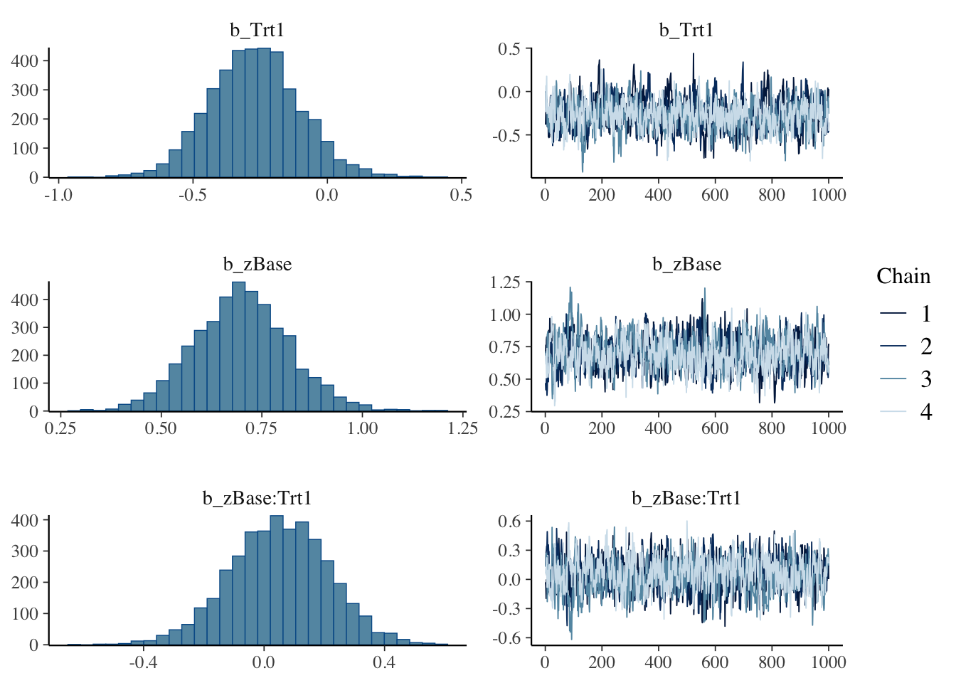
より詳しく見るにはconditional_effects関数を用いることもできる.交差項の効果はほとんどないことがわかる:

plot(conditional_effects(fit1, effects = "zBase:Trt"))
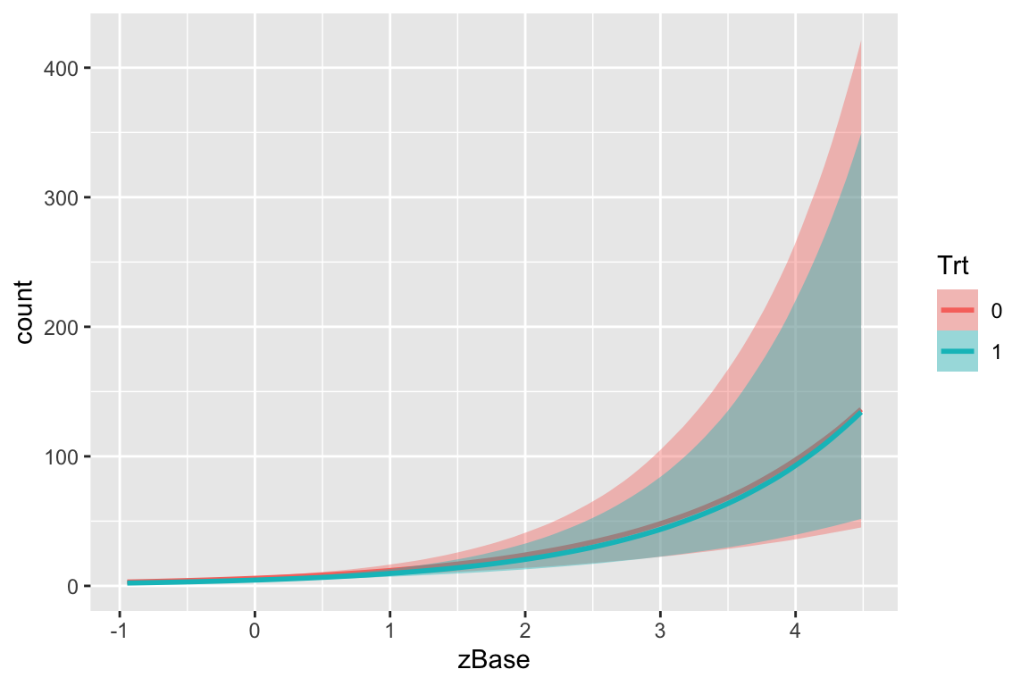
図 1

1.3 モデルによる予測

fit したモデル fit1 を用いて,平均年齢と平均ベースレートを持つ患者に対する治療効果を予測する:

newdata <- data.frame(Trt = c(0, 1), zAge = 0, zBase = 0)
predict(fit1, newdata = newdata, re_formula = NA)
     Estimate Est.Error Q2.5 Q97.5
[1,]   5.8870  2.501858    2    11
[2,]   4.5655  2.156588    1     9

関数predict()は事後予測分布からのサンプリングを行う.一方で,関数fitted()は平均を返す.

fitted(fit1, newdata = newdata, re_formula = NA)
     Estimate Est.Error     Q2.5    Q97.5
[1,] 5.905118 0.7105245 4.614680 7.413713
[2,] 4.537683 0.5298045 3.559239 5.647088

従って,もう1度ずつ実行すると,predictでは値が変わるが,fittedでは同じ値が出力される.

predict(fit1, newdata = newdata, re_formula = NA)
     Estimate Est.Error Q2.5 Q97.5
[1,]  5.94525  2.551251    2    12
[2,]  4.57525  2.225101    1     9
fitted(fit1, newdata = newdata, re_formula = NA)
     Estimate Est.Error     Q2.5    Q97.5
[1,] 5.905118 0.7105245 4.614680 7.413713
[2,] 4.537683 0.5298045 3.559239 5.647088

1.4 モデルの比較

モデルfit1で行った Poisson 回帰分析は,fit1に含めた説明変数の違いを除けば,個々の観測が独立になる,という仮定の上に成り立っている(第 4.3 節).

この仮定が破れているとき=全ての説明変数をモデルに含めきれていないとき,Poisson 分布の性質 \[ \operatorname{E}[X]=\mathrm{V}[X]=\lambda\qquad (X\sim\mathrm{Pois}(\lambda)) \] からの離反として現れ,この現象は 過分散(overdispersion)とも呼ばれる.

1.4.1 観測レベルランダム効果

ということで,他の説明変数が存在した場合を想定して, Poisson 分布族ではなく,分散が平均よりも大きいような別の分布族を用いて,フィット度合いを比較してみることを考えたい.

そこで,追加の変動をモデルに追加するべく,モデルfit1に観測ごとの切片項 \(\eta_{it}\) を追加してみる(この手法は観測レベルランダム効果と呼ばれる.第 3.3 節参照).

fit2 <- brm(count ~ zAge + zBase * Trt + (1|patient) + (1|obs),
            data = epilepsy, family = poisson())
fit2 <- brm(count ~ zAge + zBase * Trt + (1|patient) + (1|obs),
            data = epilepsy, family = poisson())
Compiling Stan program...
Start sampling

SAMPLING FOR MODEL 'anon_model' NOW (CHAIN 1).
Chain 1: 
Chain 1: Gradient evaluation took 7.4e-05 seconds
Chain 1: 1000 transitions using 10 leapfrog steps per transition would take 0.74 seconds.
Chain 1: Adjust your expectations accordingly!
Chain 1: 
Chain 1: 
Chain 1: Iteration:    1 / 2000 [  0%]  (Warmup)
Chain 1: Iteration:  200 / 2000 [ 10%]  (Warmup)
Chain 1: Iteration:  400 / 2000 [ 20%]  (Warmup)
Chain 1: Iteration:  600 / 2000 [ 30%]  (Warmup)
Chain 1: Iteration:  800 / 2000 [ 40%]  (Warmup)
Chain 1: Iteration: 1000 / 2000 [ 50%]  (Warmup)
Chain 1: Iteration: 1001 / 2000 [ 50%]  (Sampling)
Chain 1: Iteration: 1200 / 2000 [ 60%]  (Sampling)
Chain 1: Iteration: 1400 / 2000 [ 70%]  (Sampling)
Chain 1: Iteration: 1600 / 2000 [ 80%]  (Sampling)
Chain 1: Iteration: 1800 / 2000 [ 90%]  (Sampling)
Chain 1: Iteration: 2000 / 2000 [100%]  (Sampling)
Chain 1: 
Chain 1:  Elapsed Time: 2.09 seconds (Warm-up)
Chain 1:                1.138 seconds (Sampling)
Chain 1:                3.228 seconds (Total)
Chain 1: 

SAMPLING FOR MODEL 'anon_model' NOW (CHAIN 2).
Chain 2: 
Chain 2: Gradient evaluation took 1.9e-05 seconds
Chain 2: 1000 transitions using 10 leapfrog steps per transition would take 0.19 seconds.
Chain 2: Adjust your expectations accordingly!
Chain 2: 
Chain 2: 
Chain 2: Iteration:    1 / 2000 [  0%]  (Warmup)
Chain 2: Iteration:  200 / 2000 [ 10%]  (Warmup)
Chain 2: Iteration:  400 / 2000 [ 20%]  (Warmup)
Chain 2: Iteration:  600 / 2000 [ 30%]  (Warmup)
Chain 2: Iteration:  800 / 2000 [ 40%]  (Warmup)
Chain 2: Iteration: 1000 / 2000 [ 50%]  (Warmup)
Chain 2: Iteration: 1001 / 2000 [ 50%]  (Sampling)
Chain 2: Iteration: 1200 / 2000 [ 60%]  (Sampling)
Chain 2: Iteration: 1400 / 2000 [ 70%]  (Sampling)
Chain 2: Iteration: 1600 / 2000 [ 80%]  (Sampling)
Chain 2: Iteration: 1800 / 2000 [ 90%]  (Sampling)
Chain 2: Iteration: 2000 / 2000 [100%]  (Sampling)
Chain 2: 
Chain 2:  Elapsed Time: 1.918 seconds (Warm-up)
Chain 2:                1.139 seconds (Sampling)
Chain 2:                3.057 seconds (Total)
Chain 2: 

SAMPLING FOR MODEL 'anon_model' NOW (CHAIN 3).
Chain 3: 
Chain 3: Gradient evaluation took 1.9e-05 seconds
Chain 3: 1000 transitions using 10 leapfrog steps per transition would take 0.19 seconds.
Chain 3: Adjust your expectations accordingly!
Chain 3: 
Chain 3: 
Chain 3: Iteration:    1 / 2000 [  0%]  (Warmup)
Chain 3: Iteration:  200 / 2000 [ 10%]  (Warmup)
Chain 3: Iteration:  400 / 2000 [ 20%]  (Warmup)
Chain 3: Iteration:  600 / 2000 [ 30%]  (Warmup)
Chain 3: Iteration:  800 / 2000 [ 40%]  (Warmup)
Chain 3: Iteration: 1000 / 2000 [ 50%]  (Warmup)
Chain 3: Iteration: 1001 / 2000 [ 50%]  (Sampling)
Chain 3: Iteration: 1200 / 2000 [ 60%]  (Sampling)
Chain 3: Iteration: 1400 / 2000 [ 70%]  (Sampling)
Chain 3: Iteration: 1600 / 2000 [ 80%]  (Sampling)
Chain 3: Iteration: 1800 / 2000 [ 90%]  (Sampling)
Chain 3: Iteration: 2000 / 2000 [100%]  (Sampling)
Chain 3: 
Chain 3:  Elapsed Time: 1.983 seconds (Warm-up)
Chain 3:                1.133 seconds (Sampling)
Chain 3:                3.116 seconds (Total)
Chain 3: 

SAMPLING FOR MODEL 'anon_model' NOW (CHAIN 4).
Chain 4: 
Chain 4: Gradient evaluation took 2.4e-05 seconds
Chain 4: 1000 transitions using 10 leapfrog steps per transition would take 0.24 seconds.
Chain 4: Adjust your expectations accordingly!
Chain 4: 
Chain 4: 
Chain 4: Iteration:    1 / 2000 [  0%]  (Warmup)
Chain 4: Iteration:  200 / 2000 [ 10%]  (Warmup)
Chain 4: Iteration:  400 / 2000 [ 20%]  (Warmup)
Chain 4: Iteration:  600 / 2000 [ 30%]  (Warmup)
Chain 4: Iteration:  800 / 2000 [ 40%]  (Warmup)
Chain 4: Iteration: 1000 / 2000 [ 50%]  (Warmup)
Chain 4: Iteration: 1001 / 2000 [ 50%]  (Sampling)
Chain 4: Iteration: 1200 / 2000 [ 60%]  (Sampling)
Chain 4: Iteration: 1400 / 2000 [ 70%]  (Sampling)
Chain 4: Iteration: 1600 / 2000 [ 80%]  (Sampling)
Chain 4: Iteration: 1800 / 2000 [ 90%]  (Sampling)
Chain 4: Iteration: 2000 / 2000 [100%]  (Sampling)
Chain 4: 
Chain 4:  Elapsed Time: 1.971 seconds (Warm-up)
Chain 4:                1.151 seconds (Sampling)
Chain 4:                3.122 seconds (Total)
Chain 4: 

こうして得た2つのモデルfit1,fit2を比較する.

LLO (Leave-One-Out) cross-validation が関数looによって実行できる:

loo(fit1, fit2)
loo(fit1, fit2)
Warning: Found 8 observations with a pareto_k > 0.7 in model 'fit1'. We
recommend to set 'moment_match = TRUE' in order to perform moment matching for
problematic observations.
Warning: Found 59 observations with a pareto_k > 0.7 in model 'fit2'. We
recommend to set 'moment_match = TRUE' in order to perform moment matching for
problematic observations.
Output of model 'fit1':

Computed from 4000 by 236 log-likelihood matrix.

         Estimate   SE
elpd_loo   -670.9 36.0
p_loo        93.2 13.7
looic      1341.7 72.1
------
MCSE of elpd_loo is NA.
MCSE and ESS estimates assume MCMC draws (r_eff in [0.4, 2.0]).

Pareto k diagnostic values:
                         Count Pct.    Min. ESS
(-Inf, 0.7]   (good)     228   96.6%   77      
   (0.7, 1]   (bad)        5    2.1%   <NA>    
   (1, Inf)   (very bad)   3    1.3%   <NA>    
See help('pareto-k-diagnostic') for details.

Output of model 'fit2':

Computed from 4000 by 236 log-likelihood matrix.

         Estimate   SE
elpd_loo   -595.2 14.0
p_loo       108.0  7.2
looic      1190.4 28.0
------
MCSE of elpd_loo is NA.
MCSE and ESS estimates assume MCMC draws (r_eff in [0.4, 1.6]).

Pareto k diagnostic values:
                         Count Pct.    Min. ESS
(-Inf, 0.7]   (good)     177   75.0%   85      
   (0.7, 1]   (bad)       52   22.0%   <NA>    
   (1, Inf)   (very bad)   7    3.0%   <NA>    
See help('pareto-k-diagnostic') for details.

Model comparisons:
     elpd_diff se_diff
fit2   0.0       0.0  
fit1 -75.7      26.5  

elpd_diff は expected log posterior density の差異を表す.fit2の方が大きく当てはまりが良いことが見て取れる.

また,WAIC (Watanabe-Akaike Information Criterion) も実装されている:

print(waic(fit1))
print(waic(fit1))
Warning: 
53 (22.5%) p_waic estimates greater than 0.4. We recommend trying loo instead.

Computed from 4000 by 236 log-likelihood matrix.

          Estimate   SE
elpd_waic   -667.4 36.1
p_waic        89.8 13.8
waic        1334.9 72.3

53 (22.5%) p_waic estimates greater than 0.4. We recommend trying loo instead. 
print(waic(fit2))
Warning: 
63 (26.7%) p_waic estimates greater than 0.4. We recommend trying loo instead.

Computed from 4000 by 236 log-likelihood matrix.

          Estimate   SE
elpd_waic   -571.4 11.9
p_waic        84.3  5.1
waic        1142.8 23.9

63 (26.7%) p_waic estimates greater than 0.4. We recommend trying loo instead. 

他にも,reloo, kfold などの関数もある.

methods(class="brmsfit")
 [1] add_criterion           add_ic                  as_draws_array         
 [4] as_draws_df             as_draws_list           as_draws_matrix        
 [7] as_draws_rvars          as_draws                as.array               
[10] as.data.frame           as.matrix               as.mcmc                
[13] autocor                 bayes_factor            bayes_R2               
[16] bridge_sampler          coef                    conditional_effects    
[19] conditional_smooths     control_params          default_prior          
[22] expose_functions        family                  fitted                 
[25] fixef                   formula                 getCall                
[28] hypothesis              kfold                   log_lik                
[31] log_posterior           logLik                  loo_compare            
[34] loo_linpred             loo_model_weights       loo_moment_match       
[37] loo_predict             loo_predictive_interval loo_R2                 
[40] loo_subsample           loo                     LOO                    
[43] marginal_effects        marginal_smooths        mcmc_plot              
[46] model_weights           model.frame             nchains                
[49] ndraws                  neff_ratio              ngrps                  
[52] niterations             nobs                    nsamples               
[55] nuts_params             nvariables              pairs                  
[58] parnames                plot                    post_prob              
[61] posterior_average       posterior_epred         posterior_interval     
[64] posterior_linpred       posterior_predict       posterior_samples      
[67] posterior_smooths       posterior_summary       pp_average             
[70] pp_check                pp_mixture              predict                
[73] predictive_error        predictive_interval     prepare_predictions    
[76] print                   prior_draws             prior_summary          
[79] psis                    ranef                   reloo                  
[82] residuals               restructure             rhat                   
[85] stancode                standata                stanplot               
[88] summary                 update                  VarCorr                
[91] variables               vcov                    waic                   
[94] WAIC                   
see '?methods' for accessing help and source code

1.4.2 患者内の相関構造のモデリング

また,fit1において,同一患者の異なる訪問の間には全く相関がないと仮定されており,これは全く非現実的な仮定をおいてしまっていると言える.2

患者内の相関構造は,brm()関数のautocor引数で指定できる(第 4.3.2 節).

例えば,全く構造を仮定しない場合は,unstrを指定する:

fit3 <- brm(count ~ zAge + zBase * Trt + (1|patient),
            autocor = ~unstr(time=visit, gr=patient),
            data = epilepsy, family = poisson())
fit3 <- brm(count ~ zAge + zBase * Trt + (1|patient),
            autocor = ~unstr(time=visit, gr=patient),
            data = epilepsy, family = poisson())
Warning: Argument 'autocor' should be specified within the 'formula' argument.
See ?brmsformula for help.
Compiling Stan program...
Start sampling

SAMPLING FOR MODEL 'anon_model' NOW (CHAIN 1).
Chain 1: 
Chain 1: Gradient evaluation took 0.000148 seconds
Chain 1: 1000 transitions using 10 leapfrog steps per transition would take 1.48 seconds.
Chain 1: Adjust your expectations accordingly!
Chain 1: 
Chain 1: 
Chain 1: Iteration:    1 / 2000 [  0%]  (Warmup)
Chain 1: Iteration:  200 / 2000 [ 10%]  (Warmup)
Chain 1: Iteration:  400 / 2000 [ 20%]  (Warmup)
Chain 1: Iteration:  600 / 2000 [ 30%]  (Warmup)
Chain 1: Iteration:  800 / 2000 [ 40%]  (Warmup)
Chain 1: Iteration: 1000 / 2000 [ 50%]  (Warmup)
Chain 1: Iteration: 1001 / 2000 [ 50%]  (Sampling)
Chain 1: Iteration: 1200 / 2000 [ 60%]  (Sampling)
Chain 1: Iteration: 1400 / 2000 [ 70%]  (Sampling)
Chain 1: Iteration: 1600 / 2000 [ 80%]  (Sampling)
Chain 1: Iteration: 1800 / 2000 [ 90%]  (Sampling)
Chain 1: Iteration: 2000 / 2000 [100%]  (Sampling)
Chain 1: 
Chain 1:  Elapsed Time: 4.102 seconds (Warm-up)
Chain 1:                2.262 seconds (Sampling)
Chain 1:                6.364 seconds (Total)
Chain 1: 

SAMPLING FOR MODEL 'anon_model' NOW (CHAIN 2).
Chain 2: 
Chain 2: Gradient evaluation took 3.9e-05 seconds
Chain 2: 1000 transitions using 10 leapfrog steps per transition would take 0.39 seconds.
Chain 2: Adjust your expectations accordingly!
Chain 2: 
Chain 2: 
Chain 2: Iteration:    1 / 2000 [  0%]  (Warmup)
Chain 2: Iteration:  200 / 2000 [ 10%]  (Warmup)
Chain 2: Iteration:  400 / 2000 [ 20%]  (Warmup)
Chain 2: Iteration:  600 / 2000 [ 30%]  (Warmup)
Chain 2: Iteration:  800 / 2000 [ 40%]  (Warmup)
Chain 2: Iteration: 1000 / 2000 [ 50%]  (Warmup)
Chain 2: Iteration: 1001 / 2000 [ 50%]  (Sampling)
Chain 2: Iteration: 1200 / 2000 [ 60%]  (Sampling)
Chain 2: Iteration: 1400 / 2000 [ 70%]  (Sampling)
Chain 2: Iteration: 1600 / 2000 [ 80%]  (Sampling)
Chain 2: Iteration: 1800 / 2000 [ 90%]  (Sampling)
Chain 2: Iteration: 2000 / 2000 [100%]  (Sampling)
Chain 2: 
Chain 2:  Elapsed Time: 4.034 seconds (Warm-up)
Chain 2:                3.134 seconds (Sampling)
Chain 2:                7.168 seconds (Total)
Chain 2: 

SAMPLING FOR MODEL 'anon_model' NOW (CHAIN 3).
Chain 3: 
Chain 3: Gradient evaluation took 4.4e-05 seconds
Chain 3: 1000 transitions using 10 leapfrog steps per transition would take 0.44 seconds.
Chain 3: Adjust your expectations accordingly!
Chain 3: 
Chain 3: 
Chain 3: Iteration:    1 / 2000 [  0%]  (Warmup)
Chain 3: Iteration:  200 / 2000 [ 10%]  (Warmup)
Chain 3: Iteration:  400 / 2000 [ 20%]  (Warmup)
Chain 3: Iteration:  600 / 2000 [ 30%]  (Warmup)
Chain 3: Iteration:  800 / 2000 [ 40%]  (Warmup)
Chain 3: Iteration: 1000 / 2000 [ 50%]  (Warmup)
Chain 3: Iteration: 1001 / 2000 [ 50%]  (Sampling)
Chain 3: Iteration: 1200 / 2000 [ 60%]  (Sampling)
Chain 3: Iteration: 1400 / 2000 [ 70%]  (Sampling)
Chain 3: Iteration: 1600 / 2000 [ 80%]  (Sampling)
Chain 3: Iteration: 1800 / 2000 [ 90%]  (Sampling)
Chain 3: Iteration: 2000 / 2000 [100%]  (Sampling)
Chain 3: 
Chain 3:  Elapsed Time: 4.157 seconds (Warm-up)
Chain 3:                2.383 seconds (Sampling)
Chain 3:                6.54 seconds (Total)
Chain 3: 

SAMPLING FOR MODEL 'anon_model' NOW (CHAIN 4).
Chain 4: 
Chain 4: Gradient evaluation took 3.8e-05 seconds
Chain 4: 1000 transitions using 10 leapfrog steps per transition would take 0.38 seconds.
Chain 4: Adjust your expectations accordingly!
Chain 4: 
Chain 4: 
Chain 4: Iteration:    1 / 2000 [  0%]  (Warmup)
Chain 4: Iteration:  200 / 2000 [ 10%]  (Warmup)
Chain 4: Iteration:  400 / 2000 [ 20%]  (Warmup)
Chain 4: Iteration:  600 / 2000 [ 30%]  (Warmup)
Chain 4: Iteration:  800 / 2000 [ 40%]  (Warmup)
Chain 4: Iteration: 1000 / 2000 [ 50%]  (Warmup)
Chain 4: Iteration: 1001 / 2000 [ 50%]  (Sampling)
Chain 4: Iteration: 1200 / 2000 [ 60%]  (Sampling)
Chain 4: Iteration: 1400 / 2000 [ 70%]  (Sampling)
Chain 4: Iteration: 1600 / 2000 [ 80%]  (Sampling)
Chain 4: Iteration: 1800 / 2000 [ 90%]  (Sampling)
Chain 4: Iteration: 2000 / 2000 [100%]  (Sampling)
Chain 4: 
Chain 4:  Elapsed Time: 4.12 seconds (Warm-up)
Chain 4:                2.316 seconds (Sampling)
Chain 4:                6.436 seconds (Total)
Chain 4: 
Warning: Bulk Effective Samples Size (ESS) is too low, indicating posterior means and medians may be unreliable.
Running the chains for more iterations may help. See
https://mc-stan.org/misc/warnings.html#bulk-ess
Warning: Tail Effective Samples Size (ESS) is too low, indicating posterior variances and tail quantiles may be unreliable.
Running the chains for more iterations may help. See
https://mc-stan.org/misc/warnings.html#tail-ess

このモデルもfit1より遥かに当てはまりが良く,fit2とほとんど同じ当てはまりの良さが見られる:

loo(fit2,fit3)
Warning: Found 59 observations with a pareto_k > 0.7 in model 'fit2'. We
recommend to set 'moment_match = TRUE' in order to perform moment matching for
problematic observations.
Warning: Found 51 observations with a pareto_k > 0.7 in model 'fit3'. We
recommend to set 'moment_match = TRUE' in order to perform moment matching for
problematic observations.
Output of model 'fit2':

Computed from 4000 by 236 log-likelihood matrix.

         Estimate   SE
elpd_loo   -595.2 14.0
p_loo       108.0  7.2
looic      1190.4 28.0
------
MCSE of elpd_loo is NA.
MCSE and ESS estimates assume MCMC draws (r_eff in [0.4, 1.6]).

Pareto k diagnostic values:
                         Count Pct.    Min. ESS
(-Inf, 0.7]   (good)     177   75.0%   85      
   (0.7, 1]   (bad)       52   22.0%   <NA>    
   (1, Inf)   (very bad)   7    3.0%   <NA>    
See help('pareto-k-diagnostic') for details.

Output of model 'fit3':

Computed from 4000 by 236 log-likelihood matrix.

         Estimate   SE
elpd_loo   -599.7 14.6
p_loo       111.2  7.7
looic      1199.5 29.2
------
MCSE of elpd_loo is NA.
MCSE and ESS estimates assume MCMC draws (r_eff in [0.4, 1.5]).

Pareto k diagnostic values:
                         Count Pct.    Min. ESS
(-Inf, 0.7]   (good)     185   78.4%   55      
   (0.7, 1]   (bad)       45   19.1%   <NA>    
   (1, Inf)   (very bad)   6    2.5%   <NA>    
See help('pareto-k-diagnostic') for details.

Model comparisons:
     elpd_diff se_diff
fit2  0.0       0.0   
fit3 -4.5       2.9   

思ったよりもfit2の当てはまりが良いため,Poisson-対数正規混合モデリングを本格的に実施してみることが,次の選択肢になり得る(第 3.3 節参照).

1.5 その他の例

Sebastian Weber らにより,新薬の治験における実際の解析事例をまとめたウェブサイト が公開されている.3

特に,13 章で,同様の経時的繰り返し観測データを扱っているが,ここではカウントデータではなく連続な応用変数が扱われている.

2 ランダム効果モデルの正しい使い方

概要
  • ランダム効果モデル とは,グループ毎に異なる切片項 \(\alpha_{s[i]}\) を追加し,これにも誤差を仮定してモデルに入れて得る階層モデルである.
  • しかし,\(\alpha_{s[i]}\) が(ユニットレベルの)説明変数 \(x_i\) と相関を持つ場合,推定量の一致性が失われる.これを回避するために,\(x_i\) の係数 \(\beta\) にのみ関心がある場合は,固定効果モデルが用いられることも多い.
  • だが,簡単なトリック(\(\alpha_{s[i]}\) の説明変数に \(\overline{x}_s\) を追加すること)で,推定量の一致性を回復することができる.
  • このトリックを取り入れたランダム効果モデルは,\(x_i\)\(\alpha_{s[i]}\) に相関がない場合は固定効果モデルと等価な \(\beta\) の推定量を与え,相関がある場合でも,\(\beta\) を一致推定し,各変動切片項 \(\alpha_{s[i]}\) の構造にも洞察を与えてくれる.

ランダム効果モデルは線型混合モデル (Linear Mixed Model; LMM) とも呼ばれる.

LMM は,母数の共通化によるデータのプーリングと変動効果による標本平均の縮小作用を生み出すことのできるモデルであり,その結果生ずる予測量が EBLUE になる.したがって,EBLUE は,各々の地域の標本平均とプールされた回帰推定量との加重平均になっており,データ数が少ないときには標本平均をプールされた推定量の方向へ縮小することにより,推定精度の改善を図っている.(久保川達也, 2006)

2.1 ランダム効果モデル

ランダム効果 は,変動する切片項と呼んだ方がわかりやすい (Bafumi and Gelman, 2007) と言われるように,サブグループ毎に異なる切片項のことである.4

ユニット(個人などの最小単位)レベルの回帰式を書き下すと,グループ選択関数 \(s:[n]\to[S]\;(S\le n)\) を通じて, \[ y_i=\alpha_{s[i]}+\beta x_i+\epsilon_i,\qquad i\in[n], \tag{1}\] というようになる.

これは,確率変数 \(\alpha_{s[i]}\) の平均を \(\alpha_0\) とすると,グループレベルの回帰式 \[ \alpha_s=\alpha_0+\eta_s,\qquad s\in[S] \tag{2}\] が背後にある 階層モデル (multilevel / hierarchical model) だとみなすこともできる.

2.2 説明変数との相関の問題

2.2.1 問題の所在

ランダム効果では,ユニットレベルの説明変数 \(x_i\) と変動切片項 \(\alpha_{s[i]}\) が相関を持たないという仮定が Gauss-Markov の定理の仮定に等価になるため,これが違反されると推定量の不偏性・一致性が約束されず,推定量の分散も大きくなる.5

Gauss-Markov の仮定

ユニットレベル回帰式 \[ y_i=\alpha_{s[i]}+\beta x_i+\epsilon_i,\qquad i\in[n],\tag{1} \] において,ユニットレベルの説明変数 \(x_i\) と変動切片項 \(\alpha_{s[i]}\) が相関を持たないこと.

実際,ランダム効果モデルの階層構造を,(2) を (1) に代入することで一つの式にまとめると \[ y_i=\alpha_0+\beta x_i+\underbrace{\epsilon_i'}_{\epsilon_i+\eta_{s[i]}} \tag{3}\] を得る.

このような誤差項の構造 \(e_{it}=\alpha_i+\epsilon_{it}\)一元配置モデル (one-way error component model) ともいう (Hansen, 2022, p. 600), (久保川達也, 2006, p. 155)

\(x_i\)\(\alpha_{s[i]}\) に相関がある場合,\(x_i\)\(\eta_s\) にも相関があるため,結果として (3) では説明変数と誤差 \(\epsilon_i'\) に相関が生じてしまう.これは計量経済学では 内生性 (endogeneity) の問題と呼ばれているものに他ならない.

2.2.2 業界の現状:母数効果モデル

そのため,ランダム効果モデルは避けられる傾向にあり,切片項 \(\alpha_{s[i]}\equiv\alpha_0\) は変動しないとし,グループレベルの効果を無視してモデリングすることも多い: \[ y_i=\alpha_0+\beta x_i+\epsilon_i. \] このことを 完全プーリングモデル (complete pooling model) または母数効果モデルと呼び,ランダム効果モデルを 部分プーリングモデル (partial pooling model) と呼んで対比させることがある.6

周辺モデル (marginal model) や 母平均モデル (population-average model) とも呼ばれる (Gardiner et al., 2009, p. 228)

実際,これ以上の仮定を置かず,ランダム効果は局外母数として(母数効果ともいう)一般化推定方程式の方法(第 2.6 節)によれば,\(\beta\) の不偏推定が可能である.

リンク関数 \(g\) を通じた非線型モデル \[ g(\operatorname{E}[y_i|x_i])=\beta x_i \] であっても,指数型分布族を仮定すれば,\(\beta\) の一致推定が可能である.

だが,切片項の変動を消してしまうことで,回帰係数 \(\beta\) の推定に対する縮小効果(第 3.2 節)が得られないという欠点もあり,小地域推定などにおいては \(\alpha_{s[i]}\) を確率変数とみなす積極的理由もある.この点については (久保川達也, 2006) も参照.

2.2.3 固定効果モデルという解決

問題を起こさずに,しかしながらグループレベルの効果をモデリングしたい場合, \[ y_i=\alpha_{s[i]}^{\text{unmodeled}}+\beta x_i+\epsilon_i \] \[ \alpha_s^{\text{unmodeled}}\sim\mathrm{N}(\alpha_0,\infty) \] として,グループ毎に変動する切片項 \(\alpha_{s[i]}^{\text{unmodeled}}\) を許すが,この変数自体にモデルは仮定しない,とすることもできる.

このようなモデルは,グループ毎に別々の回帰分析を実行し,\(\beta\) の値はこれらのグループの間で適切に重みづけて最終的な推定値としているに等しい.

すなわち,グループの数だけ,グループへの所属を表す2値変数 \(1_{s[i]=s}\) を導入し,\(S\) 個の項 \(\sum_{s=1}^S1_{s[i]=s}\alpha_{s[i]}^{\text{unmodeled}}\) を説明変数に加えて回帰分析を行うことに等しい.

固定効果モデルの別名
  • (Hansen, 2022) をはじめ,計量経済学では fixed effects model と呼ばれる.
  • (Bafumi and Gelman, 2007) は unmodeled varying intercept と呼んでいる.
  • least squares dummy variable regression とも呼べる.7

2.3 固定効果 vs. 変量効果

利点

\(x_i\)\(\alpha_{s[i]}\) が相関を持ち得る場合も,固定効果モデルでは問題が生じない.8

問題点

異なるグループのデータが相互作用する機構がランダム効果モデルに比べて貧しい.

例えばランダム効果モデルを用いた場合,外れ値グループが存在するなどノイズの大きなデータに対しても,\(\eta_s\) を通じて緩やかに情報が伝達され,\(\beta\) の値は平均へ縮小されて推定される(第 3.2 節).固定効果モデルではそのような頑健性を持たない (Bafumi and Gelman, 2007, pp. 4–5)

固定効果モデルは \(\beta\) (のみ)に関心がある場合,\(\alpha_{s[i]}\)\(x_i\) の相関の存在に対してロバストな推定法として有用であり,その理由で計量経済学(特に線型パネルデータ)では主流の推定手法となっている.9

実際,\(\alpha_{s[i]}\)\(x_i\) が無相関であるとき,変量効果モデルと固定効果モデルは \(\beta\) に関しては等価な推定量を与える.

Current econometric practice is to prefer robustness over efficiency. Consequently, current practice is (nearly uniformly) to use the fixed effects estmimator for linear panel data models. (Hansen, 2022, p. 624)

逆に言えば,固定効果モデルは \(x_i\)\(\alpha_{s[i]}\) の構造のモデリングを放棄したモデリング法であり,各 \(\alpha_{s[i]}\) の値にも興味がある場合,または \(\beta\) のより精度の高い推定が実行したい場合には,やはり \(\alpha_{s[i]}\) の誤差と相関構造もモデルに取り入れたランダム効果モデルを用いたいということになる.

2.4 ランダム効果モデルにおける相関のモデリング

\(x_i\)\(\alpha_{s[i]}\) が相関を持つ場合に一致推定が保証されないことがランダム効果モデルの欠陥だと述べたが,実はこれは簡単な方法で解決できる.

\(x_i\)\(\alpha_{s[i]}\) との相関は,欠落変数が存在するため,と考えることができる.

そしてこの相関は,説明変数の平均 \(\overline{x}_s\) を変動する切片項 \(\alpha_s\) の説明変数として追加することで除去できる:10

\[ y_i=\alpha_{s[i]}+\beta x_i+\epsilon_i \] \[ \alpha_s=\alpha_0+\alpha_1\overline{x}_s+\eta_s \]

これにより,Gauss-Markov の仮定(外生性)が回復される.

(Bafumi and Gelman, 2007, pp. 7–9) にシミュレーションによる検証が掲載されている.

Practitioners can get around this problem by taking advantage of the multilevel structure of their regression equation. (Bafumi and Gelman, 2007, p. 12)

2.5 第三の名前:混合効果モデル

以上,解説してきたランダム効果モデル/変量効果モデルであるが,混合効果モデル とも呼ばれる.11

何を言っているのかわからないかもしれないが,式 (1) \[ y_i=\alpha_{s[i]}+\beta x_i+\epsilon_i,\qquad i\in[n],\tag{1} \] において,\(\alpha_{s[i]}\) がランダム効果であるが,回帰係数 \(\beta\)固定効果 とも呼ぶことがあるのである.

そしてこう見ると全体として固定効果と変量効果が同居した 混合(効果)モデル とも呼べそうである.

現代的には,必要ならば \(\beta\) を確率変数とみなしても良いだろうが,慣習的にそう呼ぶため,これに従わざるを得ない,というのが (Hansen, 2022, p. 625) などを見る限り共通了解であるようである.

これが計量経済学における固定効果モデル(第 2.2.3 節)の名前の由来である.12 実際,固定効果モデルは,たしかに(ユニットレベルでの回帰係数という意味での)「固定効果」を表す変数しか含んでいない(少なくとも見た目上は).

線型混合モデルの別名

式 (1) \[ y_i=\alpha_{s[i]}+\beta x_i+\epsilon_i,\qquad i\in[n],\tag{1} \] で定義されるモデルは,(Chung et al., 2013) によると次のような複数の名前を持つ:

  • 線型混合モデル (linear mixed models) (Kincaid, 2005)
  • 階層モデル (hierarchical models)
  • マルチレベル線型モデル (multilevel linear models)
  • 混合効果モデル (mixed-effects models) (Chung et al., 2015)
  • ランダム効果モデル (random effects model) (Hubbard et al., 2010)(Bafumi and Gelman, 2007)
  • 分散成分モデル (variance component model)13

2.6 GEE との違い

一般化推定方程式 (GEE: Generalized Estimating Equation) では,ランダム効果モデルにおける階層的な議論を全て「局外母数」として捨象し,母数 \(\beta\) の推定に集中する見方をする.

GEE との違い
  1. 回帰式が違う

    線型の場合の GEE は \[ Y_{it}=\alpha+\beta_1x_{1,i,t}+\cdots+\beta_px_{p,i,t} \] とも表され,ランダムな切片項というものは見当たらない.その代わり,グループ間の影響は相関係数行列としてモデル化を行う.ランダム効果モデルでは,この相関構造をランダムな切片項を追加することで表現し,回帰式を複数立てることでモデルを表現する.

  2. 推定目標が違う

    GEE は population average model でよく用いられる (Hubbard et al., 2010) ように,あくまで応答 \(Y_{it}\) の平均の不偏推定が目標であり,共分散構造はいわば局外母数である.一方,混合効果モデルは,その階層モデルとしての性質の通り,平均構造と分散構造のいずれも推定対象として扱う志向性がある.

  3. 推定方法が違う

    混合効果モデルは主に最尤法により推定される (Hubbard et al., 2010).GEE はモーメント法により推定され,最尤法ベースではないため,完全にランダムとは言えない欠測がある場合は弱く,欠測データに対しては IPW などの方法が用いられる.

GEE にとって相関構造は局外母数であり,正確な特定は目的に含まれない.この意味で GEE の相関係数⾏列におく仮定は「間違えていてもよい便宜的な仮定」であるため,作業相関係数行列 (working correlation coefficient matrix) とも呼ばれる.相関構造を誤特定していても,平均構造は一致推定が可能であり,ロバストである.両方の特定に成功した場合はセミパラメトリック有効性が達成される.

一方で混合効果モデルは,階層モデルとして平均構造と分散構造のいずれにも明示的な仮定をおくため,片方(例えば共分散構造)の特定を間違えていた場合,もう片方の解釈性が失われる,というリスクがあると論じることができる.特に (Hubbard et al., 2010) に見られる論調である.

しかし小地域推定や,「子供の身長の成長曲線の描画」が主な研究目的である場合など,ユニットの平均効果ではなく個別効果に注目したい場合には混合効果モデルの方が適していることになる (Gardiner et al., 2009).実際,モデルの特定に成功していれば,いずれのパラメータも最尤推定されるため,一致性を持つ.

従って,モデル選択において用いられる基準も違う.GEE における作業相関係数行列と説明変数の選択には QIC (Quasi-likelihood Information Criterion) が,混合効果モデルには AIC や BIC (または cAIC や mAIC (Vaida and Blanchard, 2005))が用いられる (Gardiner et al., 2009, p. 228)

2.7 ベイズ混合効果モデルという光……?

しかし,結局ベイズ統計学の立場からは,2つの違いはほとんど重要ではなく,混合効果モデルを推定した後に,周辺化をして平均構造に関する marginal estimator を構成すれば,GEE の代用になっているのではないか?

計算機の性能と,計算統計手法の発展が目まぐるしい現代にて,過去の議論を踏襲しすぎることは,問題の本質を誤るということもあるのだろう.

ということで,以上議論したグループレベル構造を持ったデータに対する2階の階層モデルを,本稿では「混合効果モデル」と呼ぶことにする.

この節はこれで終わり.

3 混合効果モデリングのテクニック集

概要
  • 混合効果モデルの推定において,グループレベル変動 \(\alpha_{s[i]}\) の共分散行列 \(\mathrm{V}[\eta_s]\) の推定が不安定になり得る.特に,グループ数 \(S\) が小さい場合に顕著である.
  • カウントデータの Poisson モデルでは,「観測レベルのランダム効果」を追加することで,実質的に Poisson-対数正規混合モデリングを実行できる.

3.1 グループレベル分散の推定

3.1.1 問題

混合効果モデル(階層モデル) \[ y_i=\alpha_{s[i]}+\beta x_i+\epsilon_i,\qquad i\in[n],\tag{1} \] の推定において,特にグループ数 \(S\) が小さい場合,グループレベルの変動切片項 \(\alpha_{s[i]}\) の共分散行列 \(\mathrm{V}[\eta_s]\) の推定が不安定になったり,分散が負の値をとったりするという問題点が古くからある (Harville, 1977)14

変量効果 \(\eta_s\)\(\eta_s\overset{\text{iid}}{\sim}(0,\sigma^2_s)\),誤差を \(\epsilon_i\overset{\text{iid}}{\sim}(0,\sigma^2_e)\) とすると,この \(\mathrm{V}[\eta_s]\) は次の形をもち,グループ間の相関構造のモデリングを一手に引き受けている: \[ \mathrm{V}[\eta_{s}]=\sigma^2_sJ_{n_s}+\sigma_e^2I_{n_s},\qquad J_{n_s}:=\boldsymbol{1}_{n_s}\boldsymbol{1}_{n_s}^\top. \]

EM アルゴリズムが提案されたばかりの頃 (Laird and Ware, 1982) では,共分散構造にパラメトリックな仮定をおいていたが,現代ではこれを取り去った最尤推定法・ベイズ推定法が主流である.

3.1.2 退化しない共分散行列推定

しかし,最尤推定法と,一定の事前分布を仮定したベイズ MAP 推定法では,推定された共分散行列が退化してしまったり,分散が負の値を取ってしまうことがある.

打ち切り推定量 (T. Kubokawa and Srivastava, 1999), (Tatsuya Kubokawa, 2000) なども提案されているが,ベイズでは Wishart 事前分布を仮定することでこれが回避される (Chung et al., 2015)15 これは最尤法の文脈では,penalized likelihood と等価になる (Chung et al., 2013)

モデルのサイズによっては,完全なベイズ推定を実行することが難しく,一部は等価な頻度論的な方法や近似を用いることもある.その際,最適化ソルバーの収束を速めるために,共分散構造に(データや計画とは無関係に)パラメトリックモデルを仮定してしまうこともある (Kincaid, 2005)

3.2 係数の縮小推定

分散 \(\mathrm{V}[\eta_s]\) を推定して分散比 \(\rho:=\sigma_v^2/\sigma_e^2\) の推定量 \(\widehat{\rho}\) を得て,これを最良線型不偏推定量 (BLUE) \(\widehat{\beta}\) に代入して得られる,グループごとの \(y_s\) の推定量に \[ \widehat{y}_s:=\frac{\widehat{\rho}n_s}{1+\widehat{\rho}n_s}\overline{y}_s+\frac{1}{1+\widehat{\rho}n_s}\overline{x}_s^\top\widetilde{\beta}(\widehat{\rho}) \] というものがあり,これを 経験 BLUE という (久保川達也, 2006, p. 143)

これは,各グループ \(s\in[S]\) における値 \(y_s\) を,単なる経験平均 \(\overline{y}_s\) ではなく,全データプールから得られる推定量 \(\overline{x}_s^\top\widetilde{\beta}(\widehat{\rho})\) で補正した推定量になっている.

このことにより,各グループ \(s\in[S]\) のデータ数が少なく,経験平均 \(\overline{y}_s\) では分散が大きくなってしまう場合でも,安定した推定量を得ることができる.

縮小推定は小地域推定 (George E. Battese and Fuller, 1988) に応用を持つ.例えば \(s\in[S]\) をアメリカ合衆国の各州とし,投票行動のデータに応用した例が (Gelman, 2014) にある.

このように,変量効果 \(\alpha_{s[i]}\) を追加したモデリングを実行することにより,グループごとの被説明変数を縮小推定することができる.

3.2.1 経験ベイズ

縮小推定の効用は初め,経験ベイズの枠組みで説明された.

以上の考え方は,経験ベイズの枠組みで (Efron and Morris, 1975) の一連の論文の中で示されてきたものであり,ベイズ的アプローチの現実的な有用性は基本的には上述の考え方に基づいている.

そもそも1元配置混合線型モデルは \[ y_{ij}=\theta_{ij}+e_{ij},\qquad \theta_{ij}=x_{ij}^\top\beta+v_i \] とも理解できる.これは階層モデル \[ y_{ij}\sim\mathrm{N}(\theta_{ij},\sigma^2_e),\qquad\theta_{ij}\sim\mathrm{N}(x_{ij}^\top\beta,\sigma_v^2) \] とも見れる.

\(\beta,\sigma^2_v,\sigma^2_e\) を未知母数として扱った場合を 経験ベイズモデル,変量として扱って更なる分布を仮定した場合を(狭義の) 階層ベイズ ともいう (久保川達也, 2006, p. 155)

3.3 カウントデータ過分散へのお手軽対処法

これはカウントデータのモデリング限定のテクニックである.

カウントデータも,一般化線型(混合)モデルの範疇で扱うことができるため,リンク関数 \(g\) を通じてほとんど同等の扱いが可能である.

3.3.1 負の二項分布によるモデリング

カウントデータの基本は Poisson 分布であろうが,過分散を考慮するために,負の二項分布でモデリングすることもできる.負の二項分布は例えばマーケティングにおいて,顧客の購買回数をモデル化する際に用いられる (森岡毅,今西聖貴, 2016)

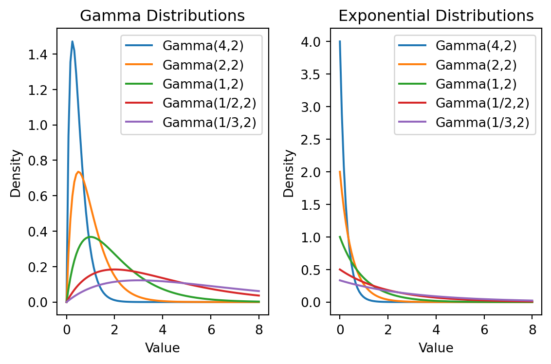
この行為は,Poisson 分布の Gamma 分布による混合分布族を用いた,混合モデリングを行っているとみなせる:

命題

Poisson 分布 \(\mathrm{Pois}(\theta)\)\(\mathrm{Gamma}(\alpha,\nu)\)-混合は負の二項分布 \(\mathrm{NB}\left(\nu,\frac{\alpha}{\alpha+1}\right)\) になる.

ただし,負の二項分布 \(\mathrm{NB}(\nu,p)\) は,次の確率質量関数 \(p(x;\nu,p)\) が定める \(\mathbb{N}\) 上の確率分布である: \[ p(x;\nu,p)=\begin{pmatrix}x+\nu-1\\x\end{pmatrix}p^\nu(1-p)^x. \]

確率分布の変換則より,次のように計算できる:

\[\begin{align*} p(x)&=\int_{\mathbb{R}_+}\frac{\theta^x}{x!}e^{-\theta}\frac{1}{\Gamma(\nu)}\alpha^\nu\theta^{\nu-1}e^{-\alpha\theta}d\theta\\ &=\frac{\alpha^\nu}{x!\Gamma(\nu)}\int_{\mathbb{R}_+}\theta^{x+\nu-1}e^{-(\alpha+1)\theta}d\theta\\ &=\frac{\alpha^\nu}{x!\Gamma(\nu)}\frac{\Gamma(x+\nu)}{(\alpha+1)^{x+\nu}}\\ &=\begin{pmatrix}\nu+x-1\\x\end{pmatrix}\left(\frac{1}{\alpha+1}\right)^x\left(\frac{\alpha}{\alpha+1}\right)^\nu. \end{align*}\]

この最右辺は,たしかに負の二項分布の質量関数である.

この証明方法と,Gamma 分布については次の記事を参照:

Article Image

確率測度の変換則

Gamma 分布とBeta 分布を例に

これは \[ y_{it}\sim\mathrm{Pois}(\theta) \] \[ \theta\sim\mathrm{Gamma}(\alpha,\nu) \] という Gamma 分布を仮定した経験ベイズモデル(第 3.2.1 節)に当たる.

Gamma 分布は Poisson 分布の共役事前分布であるため計算が容易であり,早くから質病地図の作成などにも用いられていた (Clayton and Kaldor, 1987), (丹後俊郎, 1988)

3.3.2 Poisson-対数正規混合によるモデリング

Poisson 回帰

\[ \begin{align*} y_{it} & \sim \operatorname{Pois}(\lambda_{s[i]}) \\ \log(\lambda_{s[i]}) & = \alpha_i + \eta_{it} \\ \eta_{it} & \sim \operatorname{N}(0, \sigma). \end{align*} \]

を考えると,各 \(y_{it}\) を,(グループ毎に条件付ければ)Poisson 分布の対数正規分布による混合分布を用いてモデル化していることにあたる.

この,Poisson-対数正規分布族は,(Bulmer, 1974) により生物種の個体数分布のモデリングで,過分散を説明するために用いられている.

すなわち,第 1.1 節のモデルの比較 1.4 で扱った,観測レベルランダム効果 (OLRE: Observation-level Random Effects) の方法は,観測毎に \(\eta_{it}\) というランダム切片項を追加するだけで,本質的には Poisson-対数正規混合モデリングを実施する という,いわばハックのような使い方である.16

今回はモデル比較の結果が良かったため,本格的に対数正規混合を実施してみるのも良いかもしれない.

3.4 変量係数モデルによる非線型モデリング

前節 3.3 では,カウントデータに適用するための一般化線型混合モデルをみた.

(久保川達也, 2006) では,ここまで考慮した1元配置混合線型モデルの拡張をいくつか紹介している:

  • 各グループ \(s\in[S]\) の中でもいくつかのクラスターに分けられる場合,2元配置混合モデル が考えられる: \[ y_{ijk}=x_{ijk}^\top\beta+v_i+u_{ij}+e_{ijk}. \]
  • 誤差分散が一定であるという仮定が怪しい場合,変動分散モデル が考えられる.これは,グループ内の分散を \(e_{ij}|\sigma_i^2\sim\mathrm{N}(0,\sigma_i^2)\) とし,\(\sigma_i\) をグループ内で同一の分布に従う i.i.d. と仮定した階層モデルをいう.
  • 係数 \(\beta\) にもモデルを仮定した階層モデルは 変量係数モデル ともいう: \[ \beta_i=W_i\alpha+v_i. \] 州ごとの,収入因子が投票行動に与える影響の差を突き止めた (Gelman, 2014) ではこの変量係数モデルを用いている.

3.4.1 例:投票行動の州ごとの違い

(Gelman, 2014) では州ごとの投票行動の違いを説明するために,まずは次のロジスティック混合モデルを考えている: \[ \operatorname{Pr}(y_i=1)=\operatorname{logit}^{-1}(\alpha_{s[i]}+x_i\beta) \] \[ \alpha_s=W_s^\top\gamma+\epsilon_s,\qquad\epsilon_s\overset{\text{iid}}{\sim}\mathrm{N}(0,\sigma^2_\alpha). \]

  • \(y_i\in\{0,1\}\) は共和党に投票したか,民主党に投票したかを表す2値変数.
  • \(x_i\in\{\pm2,\pm1,0\}\) は収入のレベルを5段階で表す離散変数.
  • \(W_j\) は各州の共変量のベクトル.

しかしこのままではモデルの当てはまりが良くなかった.これは州ごとに収入が投票に与える影響が異なるためであった.これを考慮するために,(Gelman, 2014) は変量係数モデルを用いた.

3.4.2 混合モデルの変量係数モデル化

\(\beta\) を州ごとに変化させ,これに \[ \beta_s=W_s^\top\gamma'+\epsilon'_s,\qquad \epsilon'_s\overset{\text{iid}}{\sim}\mathrm{N}(0,\sigma^2_\beta), \] というモデルをおく.これにより,州ごとに変化する収入-投票関係をモデリングできる.

3.4.3 非線型モデル化

これに加えて,\(\beta_s\) を収入カテゴリのアイテム \(x_i\in\{\pm2,\pm1,0\}\) ごとに変化させることも考えられる.

これは値も持つダミー変数 \[ \boldsymbol{x}_i^j=(j-3)1_{\left\{x_i=j\right\}},\qquad j\in\{1,2,3,4,5\}, \] を成分にもつ \(\boldsymbol{x}_i\in\mathbb{Z}^5\) を用いて, \[ \operatorname{Pr}(y_i=1)=\operatorname{logit}^{-1}(\alpha_{s[i]}+\boldsymbol{x}_i^\top\boldsymbol{\beta}_s) \]

というモデルを考えることにあたる.

4 brmsの実装

brm 関数(コードは こちら)の実装を調べる.

Stan コードを扱っている関数は .stancode() であった.最終的に,.compile_model_rstan().fit_model_rstan() が呼ばれるようになっている.

4.1 事前分布

brm関数 では,デフォルトでは無情報事前分布が用いられる.

Default priors are chosen to be non or very weakly informative so that their influence on the results will be negligible and you usually don’t have to worry about them. However, after getting more familiar with Bayesian statistics, I recommend you to start thinking about reasonable informative priors for your model parameters: Nearly always, there is at least some prior information available that can be used to improve your inference.
brm(): Fit Bayesian Generalized (Non-)Linear Multivariate Multilevel Models

4.2 回帰式

brm()関数の第一引数は,validate_formula関数に渡される.

この関数は S3 のメソッドのディスパッチを用いて実装されており,brmsformulaオブジェクトに対しては,validate_formula.brmsformula関数が呼び出される.

ここではautocor引数が引かれている場合,出力のformula属性に追加される:17

fit3$formula
count ~ zAge + zBase * Trt + (1 | patient) 
autocor ~ unstr(time = visit, gr = patient)

なお,brmsformulaオブジェクトのコンストラクタは brmsformula()関数 である.これは,R のformulaオブジェクトを通じて,階層モデルを定義できるようになっている(実装はリスト).

4.3 共分散構造

共分散構造は2つの観点から,brmsformulaオブジェクトから自動的に指定される.

1つ目がグルーピング構造(共分散行列のブロック構造)であり,これはgr関数 が使用される.

2つ目がグループ内の相関構造であり,これはbrm()関数のautocor引数を用いる.

4.3.1 gr関数

この関数はbrm関数の第一引数として与えられたモデル定義式から,暗黙のうちに内部で呼び出される.

例えば,回帰式に(1|patient)が含まれていた場合,gr(patient)が呼び出される.

共分散構造におく仮定について,重要なデフォルト設定が2つある:

  • グループ間の相関構造は想定されている:cor=True

    If TRUE (the default), group-level terms will be modelled as correlated.
    gr(): Set up basic grouping terms in brms

  • 一方で,グループ内の相関構造は想定されておらず,独立とされている.具体的に指定したい場合は引数covを用いる.

    By default, levels of the same grouping factor are modeled as independent of each other.
    gr(): Set up basic grouping terms in brms

すなわち,\(\mathrm{V}[\eta_s]\) には一切仮定が置かれておらず(第 3.1 節),一方で \(\{\epsilon_{it}\}_{t=1}^T\) は互いに独立とされている.

また,この二階層目の分布族(第 2.1 節での \(\alpha_i\)\(\eta_{it}\))は,分散共分散行列 \(\mathrm{V}[\eta_s]\) を持った正規分布がデフォルトで,現状他の分布族は指定できないでいる.

dist: Name of the distribution of the group-level effects. Currently “gaussian” is the only option.
gr(): Set up basic grouping terms in brms

4.3.2 autocor引数

brm()関数には,autocor引数 が用意されている.

gr()のデフォルト値では独立とされていたグループ内の相関構造を,具体的に指定するのに用いられる.

  • unstr:一才の仮定を置かない.
  • AR:一次の自己相関構造.

4.4 推論エンジン

brm関数 は,Stan による MCMC サンプリングを通じて,事後分布を計算する.

5 文献紹介

ここでは計量経済学の呼称に従い,固定効果モデルと変量効果モデルと呼んだが,同じモデルを母数モデル (fixed effect model) と変量モデル (random effect model) と呼んだりもする (足立浩平, 2000)

6 Acknowledgements

I would like to extend my gratitude to Robert Long, who kindly shared me the knowledge about the covariance structure implicitly defined via brms formula on this Cross Validated post. His insights were instrumental in enhancing this work.

References

Bafumi, J., and Gelman, A. (2007). Fitting Multilevel Models When Predictors and Group Effects Correlate. SSRN.
Bulmer, M. G. (1974). On fitting the poisson lognormal distribution to species-abundance data. Biometrics, 30(1), 101–110.
Bürkner, P.-C. (2017). Brms: An r package for bayesian multilevel models using stan. Journal of Statistical Software, 80(1), 1–28.
Bürkner, P.-C. (2018). Advanced Bayesian Multilevel Modeling with the R Package brms. The R Journal, 10(1), 395–411.
Bürkner, P.-C. (2021). Bayesian item response modeling in r with brms and stan. Journal of Statistical Software, 100(5), 1–54.
Chung, Y., Gelman, A., Rabe-Hesketh, S., Liu, J., and Dorie, V. (2015). Weakly informative prior for point estimation of covariance matrices in hierarchical models. Journal of Educational and Behavioral Statistics, 40(2), 136–157.
Chung, Y., Rabe-Hesketh, S., Dorie, V., Gelman, A., and Liu, J. (2013). A nondegenerate penalized likelihood estimator for variance parameters in multilevel models. Psychometrika, 78(4), 685–709.
Clayton, D., and Kaldor, J. (1987). Empirical bayes estimates of age-standardized relative risks for use in disease mapping. Biometrics, 43(3), 671–681.
Cunningham, S. (2021). Causal inference : The mixtape. Yale University Press.
Efron, B., and Morris, C. (1975). Data analysis using stein’s estimator and its generalizations. Journal of the American Statistical Association, 70(350), 311–319.
Gardiner, J. C., Luo, Z., and Roman, L. A. (2009). Fixed effects, random effects and GEE: What are the differences? Statistics in Medicine, 28(2), 221–239.
Gelman, A. (2014). How Bayesian Analysis Cracked the Red-State, Blue-State Problem. Statistical Science, 29(1), 26–35.
George E. Battese, R. M. H., and Fuller, W. A. (1988). An error-components model for prediction of county crop areas using survey and satellite data. Journal of the American Statistical Association, 83(401), 28–36.
Hansen, B. E. (2022). Econometrics. Princeton University Press.
Harville, D. A. (1977). Maximum likelihood approaches to variance component estimation and to related problems. Journal of the American Statistical Association, 72(358), 320–338.
Hubbard, A. E., Ahern, J., Fleischer, N. L., Laan, M. V. der, Lippman, S. A., Jewell, N., … Satariano, W. A. (2010). To GEE or not to GEE: Comparing population average and mixed models for estimating the associations between neighborhood risk factors and health. Epidemiology, 21(4).
Kincaid, C. D. (2005). Guidelines for Selecting the Covariance Structure in Mixed Model Analysis. In SAS user group international,Vol. 30, pages 198–30.
Kubokawa, Tatsuya. (2000). ESTIMATION OF VARIANCE AND COVARIANCE COMPONENTS IN ELLIPTICALLY CONTOURED DISTRIBUTIONS. JOURNAL OF THE JAPAN STATISTICAL SOCIETY, 30(2), 143–176.
Kubokawa, T., and Srivastava, M. S. (1999). Improved nonnegative estimation of multivariate components of variance. The Annals of Statistics, 27(6), 2008–2032.
Laird, N. M., and Ware, J. H. (1982). Random-effects models for longitudinal data. Biometrics, 38(4), 963–974.
Leppik, I. E., Dreifuss, F. E., Porter, R., Bowman, T., Santilli, N., Jacobs, M., … Gutierrez, A. (1987). A controlled study of progabide in partial seizures. Neurology, 37(6), 963–963.
Thall, P. F., and Vail, S. C. (1990). Some covariance models for longitudinal count data with overdispersion. Biometrics, 46(3), 657–671.
Vaida, F., and Blanchard, S. (2005). Conditional akaike information for mixed-effects models. Biometrika, 92(2), 351–370.
Vehtari, A., Gelman, A., Simpson, D., Carpenter, B., and Bürkner, P.-C. (2021). Rank-Normalization, Folding, and Localization: An Improved \(\widehat{R}\) for Assessing Convergence of MCMC (with Discussion). Bayesian Analysis, 16(2), 667–718.
丹後俊郎. (1988). 死亡指標の経験的ベイズ推定量について. 応用統計学, 17(2), 81–96.
久保川達也. (2006). 線形混合モデルと小地域の推定. 応用統計学, 35(3), 139–161.
森岡毅,今西聖貴. (2016). 確率思考の戦略論―USJでも実証された数学マーケティングの力. 角川書店.
足立浩平. (2000). 計量多次元展開法の変量モデル. 行動計量学, 27(1), 12–23.

Footnotes

  1. R を最新バージョン 4.3.1 → 4.4.0 にアップデートしなければインストールに失敗したことに注意.↩︎

  2. 通常は時間的に離れている観測は相関が薄いとしても,直近の観測と関連性が高いだろう.↩︎

  3. Statistical Modeling, Causal Inference, and Social Science における こちらのエントリ も参照.↩︎

  4. すなわち,ある確率変数の従う項と考えており,変量効果 とも呼ばれる.一方で未知母数とみなす場合は 母数効果 ともいう (久保川達也, 2006)↩︎

  5. (Hansen, 2022, p. 333) 第12.3節,(Bafumi and Gelman, 2007, p. 3), (Hansen, 2022, p. 604)(Gardiner et al., 2009, p. 228)↩︎

  6. (Bafumi and Gelman, 2007, p. 5)(久保川達也, 2006, p. 141) も参照.↩︎

  7. (Bafumi and Gelman, 2007, p. 5)(Hansen, 2022, p. 609) 17.11節 など.狭義では,fixed effects model は within transformation を行い,グループ間の影響を引いたあとに回帰を実行する……という手続きを指すこともあるが,2つは等価な結果を生む.詳しくは (Cunningham, 2021) なども参照.↩︎

  8. (Hansen, 2022, p. 624) 17.25節.↩︎

  9. (Hansen, 2022, p. 624)(Bafumi and Gelman, 2007, p. 6)↩︎

  10. (Bafumi and Gelman, 2007, p. 6)↩︎

  11. (Hubbard et al., 2010) では両方の名前で呼んでいる.↩︎

  12. (Hansen, 2022, p. 625) 17.25節.疫学・生物統計学では,実験計画法でしか「固定効果」「変量効果モデル」とは言わない,という認識であることも筆者は聞いたことがある.↩︎

  13. \(\mathrm{V}[\eta_s]\) はブロック行列の構造を持つためこう呼ばれる.(久保川達也, 2006, p. 141) でも LMM と併記されている.↩︎

  14. (Laird and Ware, 1982)(Chung et al., 2013)(Chung et al., 2015)Statistical Modeling, Causal Inference, and Social Science ブログ 6/2/2023↩︎

  15. 逆 Wishart ではないらしい (Chung et al., 2015)↩︎

  16. Solomon Kurtz (2021) による解説,RPubs も参照.↩︎

  17. Line 1363↩︎