SDE のベイズ推定入門
YUIMA と Stan を用いた確率過程のベイズ推定入門
2024-05-12
A Blog Entry on Bayesian Computation by an Applied Mathematician
$$
$$
RStan は Rcpp や inline といったパッケージにより C++ を R から呼び出すことで,Stan とのインターフェイスを実現している.
一方で CmdStanR は CmdStan という Stan のコマンドラインインターフェイスを R から呼び出すことで,Stan とのインターフェイスを実現している.
RStan パッケージstan 関数RStan パッケージの本体は stan 関数である:
stan(file, model_name = "anon_model", model_code = "", fit = NA, data = list(), pars = NA, chains = 4, iter = 2000, warmup = floor(iter/2), thin = 1, init = "random", seed = sample.int(.Machine$integer.max, 1), algorithm = c("NUTS", "HMC", "Fixed_param"), control = NULL, sample_file = NULL, diagnostic_file = NULL, save_dso = TRUE, verbose = FALSE, include = TRUE, cores = getOption("mc.cores", 1L), open_progress = interactive() && !isatty(stdout()) && !identical(Sys.getenv("RSTUDIO"), "1"), ..., boost_lib = NULL, eigen_lib = NULL)model_code="" が Stan モデルを定義するコードを,文字列として直接受け渡すための引数である.
返り値はフィット済みの stanfit オブジェクトである.
他の方法は次のとおり:
file としてファイルへのパスを渡すstanfit オブジェクトを fit 引数として渡すdata:データを与える.list 型.iter:繰り返し回数.デフォルトは 2000.chains:チェイン数.デフォルトは 4.stanfit オブジェクトstan 関数は Stan モデルを C++ に変換して実行し,結果を stanfit オブジェクトとして返す.
これに対して print, summary, plot などのメソッドが利用可能である.
さらに,次の様にして MCMC サンプルを取り出すことができる:
as.array メソッドを用いて MCMC サンプルを array 型で取り出すextract メソッドを用いて MCMC サンプルを list 型で取り出すposterior ライブラリの as_draws_df メソッドを用いて MCMC サンプルを df 型で取り出す.種々のデータ型 <format> に対して as_draws_<format> が存在する.取り出した MCMC サンプルは bayesplot パッケージの mcmc_trace, mcmc_dens などの関数を用いて可視化することができる.
scode <- "
parameters {
  array[2] real y;
}
model {
  y[1] ~ normal(0, 1);
  y[2] ~ double_exponential(0, 2);
}
"
fit <- stan(model_code = scode, iter = 10000, chains = 4, verbose = FALSE)library(bayesplot)
mcmc_trace(as.array(fit), pars = c("y[1]", "y[2]"))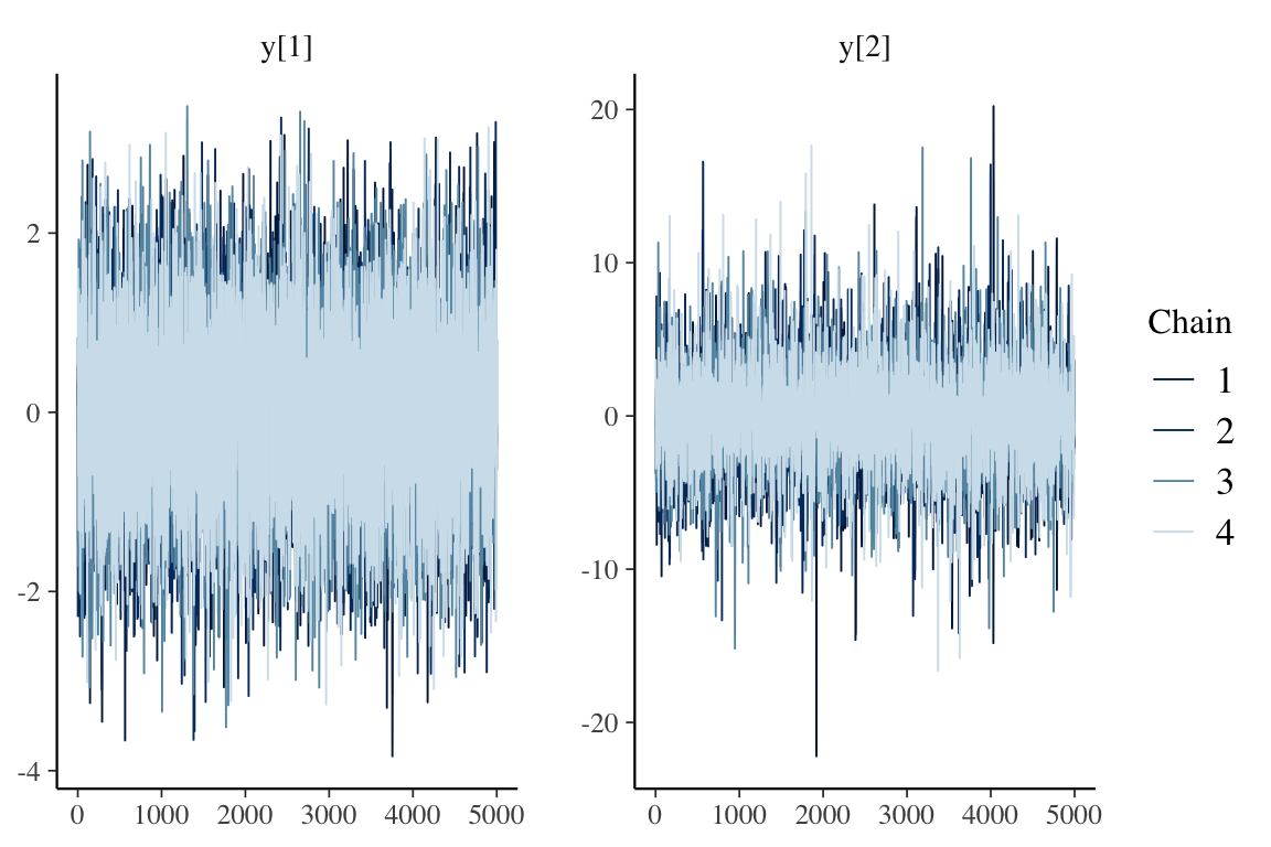
mcmc_dens(as.array(fit), pars = c("y[1]", "y[2]"))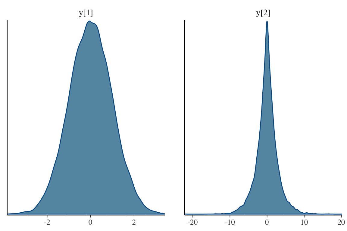
OU 過程
\[ dX_t=\theta(\mu-X_t)\,dt+\sigma\,dW_t \]
に対して,stan 関数でベイズ推定を実行してみます.
library(yuima)
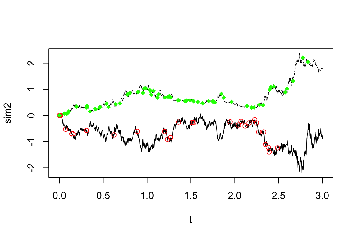
model <- setModel(drift = "theta*(mu-X)", diffusion = "sigma", state.variable = "X")パラメータは \[ \begin{pmatrix}\theta\\\mu\\\sigma\end{pmatrix} = \begin{pmatrix}1\\0\\0.5\end{pmatrix} \tag{1}\] として YUIMA を用いてシミュレーションをし,そのデータを与えてパラメータが復元できるかをみます.
library(rstan)
excode <- "data {
            int N;
            real x[N+1];
            real h;
          }

          parameters {
            real theta;
            real mu;
            real<lower=0> sigma;
          }

          model {
            x[1] ~ normal(0,1);
            for(n in 2:(N+1)){
              x[n] ~ normal(x[n-1] + theta * (mu - x[n-1]) * h,  sqrt(h) * sigma);
            }
          }"

sampling <- setSampling(Initial = 0, Terminal = 3, n = 1000)
yuima <- setYuima(model = model, sampling = sampling)
simulation <- simulate(yuima, true.parameter = c(theta = 1, mu = 0, sigma = 0.5), xinit = rnorm(1))
sde_dat <- list(N =  yuima@sampling@n,
                  x = as.numeric(simulation@data@original.data),
                  h=yuima@sampling@Terminal/yuima@sampling@n)
# シミュレーション結果
plot(simulation)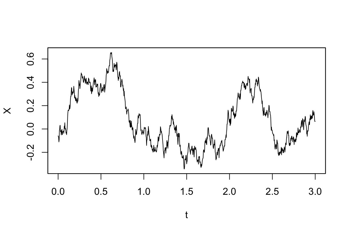
# ベイズ推定
rstan_options(auto_write = TRUE)
options(mc.cores = parallel::detectCores())

fit <- stan(model_code=excode, data = sde_dat, iter = 1000, chains = 4)print(fit)Inference for Stan model: anon_model.
4 chains, each with iter=1000; warmup=500; thin=1;
post-warmup draws per chain=500, total post-warmup draws=2000.
mean se_mean sd 2.5% 25% 50% 75% 97.5% n_eff Rhat
theta 0.79 0.07 0.93 -0.40 0.03 0.50 1.44 2.96 175 1.02
mu -0.06 0.46 3.15 -6.14 -0.68 -0.40 0.10 8.62 46 1.11
sigma 0.48 0.00 0.01 0.46 0.48 0.48 0.49 0.51 585 1.00
lp__ 3127.12 0.06 1.17 3124.36 3126.47 3127.21 3127.95 3128.86 330 1.01
Samples were drawn using NUTS(diag_e) at Sun Dec 22 10:18:54 2024.
For each parameter, n_eff is a crude measure of effective sample size,
and Rhat is the potential scale reduction factor on split chains (at
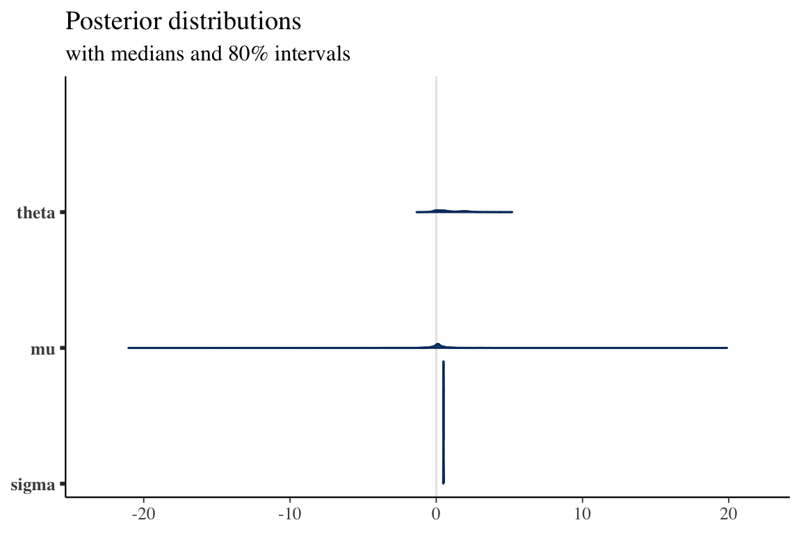
convergence, Rhat=1).パラメータ (1) がよく推定できていることがわかる.特に \(\sigma\) が安定して推定できている:
plot(fit)ci_level: 0.8 (80% intervals)outer_level: 0.95 (95% intervals)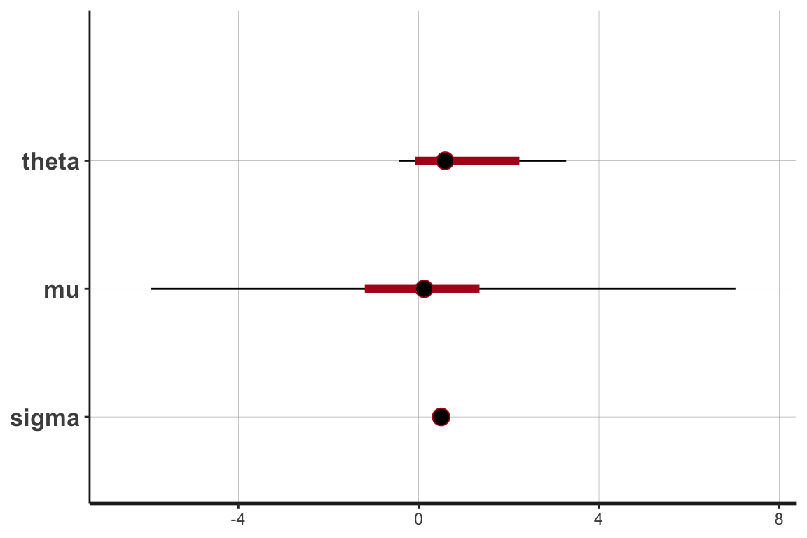
library("bayesplot")
library("rstanarm")
library("ggplot2")

posterior <- as.matrix(fit)
plot_title <- ggtitle("Posterior distributions",
                      "with medians and 80% intervals")
mcmc_areas(posterior,
           pars = c("theta", "mu", "sigma"),
           prob = 0.8) + plot_title
cmath が見つからないQuitting from lines 329-343 (adastan.qmd)
compileCode(f, code, language = language, verbose = verbose) でエラー:
using C++ compiler: ‘Apple clang version 16.0.0 (clang-1600.0.26.3)’using C++17using SDK: ‘MacOSX15.0.sdk’In file included from <built-in>:1:In file included from /Library/Frameworks/R.framework/Versions/4.3-arm64/Resources/library/StanHeaders/include/stan/math/prim/fun/Eigen.hpp:22:In file included from /Library/Frameworks/R.framework/Versions/4.3-arm64/Resources/library/RcppEigen/include/Eigen/Dense:1:In file included from /Library/Frameworks/R.framework/Versions/4.3-arm64/Resources/library/RcppEigen/include/Eigen/Core:19:/Library/Frameworks/R.framework/Versions/4.3-arm64/Resources/library/RcppEigen/include/Eigen/src/Core/util/Macros.h:679:10: fatal error: 'cmath' file not found 679 | #include <cmath> | ^~~~~~~1 error generated.make: *** [file2546221168fc.o] Error 1
呼び出し: .main ... cxxfunctionplus -> <Anonymous> -> cxxfunction -> compileCode
追加情報: 警告メッセージ:
1: パッケージ 'rstan' はバージョン 4.3.1 の R の下で造られました
2: パッケージ 'bayesplot' はバージョン 4.3.1 の R の下で造られました
3: パッケージ 'rstanarm' はバージョン 4.3.1 の R の下で造られました
Quitting from lines 329-343 (adastan.qmd)
sink(type = "output") でエラー: コネクションが不正です
呼び出し: .main ... eval -> stan -> stan_model -> cxxfunctionplus -> sink
実行が停止されました 大変長く書いてあるが,要は fatal error: 'cmath' file not found である.
筆者の場合は純粋な clang++ の問題であった:
❯ echo '#include <cmath>
#include <iostream>

int main() {
    double result = std::sqrt(16.0);
    std::cout << "The square root of 16 is " << result << std::endl;
    return 0;
}' > test.cpp


~
❯ clang++ -std=c++17 test.cpp -o test

test.cpp:1:10: fatal error: 'cmath' file not found
    1 | #include <cmath>
      |          ^~~~~~~
1 error generated.
このような場合は,まず Xcode の再インストールをすると良い.
softwareupdate --listの出力を用いて,次のようにする:
softwareupdate -i "Command Line Tools (macOS High Sierra version 10.13) for Xcode-10.1"または次のようにする:
sudo rm -rf /Library/Developer/CommandLineTools
xcode-select --installrstanarm パッケージrstanarm は他の R パッケージと同様のインターフェースで推論を実行するためのパッケージであり,MCMC の実行には rstan をバックエンドで用いる.
CmdStanR パッケージCmdStanPy, CmdStanR はいずれも Stan のインターフェースである.
CmdStanR は R6 オブジェクトを用いており,大変現代的な実装を持っている.
cmdstan_model() 関数は,Stan 言語による記述されたモデル定義を,C++ コードにコンパイルし,その結果を R6 オブジェクトとして返す.1
cmdstan_model(stan_file = NULL, exe_file = NULL, compile = TRUE, ...)返り値は CmdStanModel オブジェクトである.ただし R6 オブジェクトでもあり,R6 流のメソッドの呼び方 $ が使える.
file <- file.path(cmdstan_path(), "examples", "bernoulli", "bernoulli.stan")
mod <- cmdstan_model(file)
Stan 言語による定義は次のようにして確認できる:
mod$print()data {
int<lower=0> N;
array[N] int<lower=0, upper=1> y;
}
parameters {
real<lower=0, upper=1> theta;
}
model {
theta ~ beta(1, 1); // uniform prior on interval 0,1
y ~ bernoulli(theta);
}names(mod$variables())[1] "parameters" "included_files" "data"
[4] "transformed_parameters" "generated_quantities" names(mod$variables()$transformed_parameters)character(0)元となったファイルのパスも stan_file(), exe_file() で確認できる.
write_stan_file() 関数は Stan コードをファイルに書き出すことができる:
write_stan_file(
  code,
  dir = getOption("cmdstanr_write_stan_file_dir", tempdir()),
  basename = NULL,
  force_overwrite = FALSE,
  hash_salt = ""
)グローバル環境変数が設定されていない限り,tempdir() で一時ファイルが作成される.これは R セッションの終了とともに削除される.
stan_file_variables <- write_stan_file("
data {
  int<lower=1> J;
  vector<lower=0>[J] sigma;
  vector[J] y;
}
parameters {
  real mu;
  real<lower=0> tau;
  vector[J] theta_raw;
}
transformed parameters {
  vector[J] theta = mu + tau * theta_raw;
}
model {
  target += normal_lpdf(tau | 0, 10);
  target += normal_lpdf(mu | 0, 10);
  target += normal_lpdf(theta_raw | 0, 1);
  target += normal_lpdf(y | theta, sigma);
}
")
mod_v <- cmdstan_model(stan_file_variables)
variables <- mod_v$variables()data_list <- list(N = 10, y = c(0,1,0,0,0,0,0,0,0,1))
fit <- mod$sample(
data = data_list,
seed = 123,
chains = 4,
parallel_chains = 4,
refresh = 1000 # print update every 1000 iters
)Running MCMC with 4 parallel chains...
Chain 1 Iteration: 1 / 2000 [ 0%] (Warmup)
Chain 1 Iteration: 1000 / 2000 [ 50%] (Warmup)
Chain 1 Iteration: 1001 / 2000 [ 50%] (Sampling)
Chain 1 Iteration: 2000 / 2000 [100%] (Sampling)
Chain 2 Iteration: 1 / 2000 [ 0%] (Warmup)
Chain 2 Iteration: 1000 / 2000 [ 50%] (Warmup)
Chain 2 Iteration: 1001 / 2000 [ 50%] (Sampling)
Chain 2 Iteration: 2000 / 2000 [100%] (Sampling)
Chain 3 Iteration: 1 / 2000 [ 0%] (Warmup)
Chain 3 Iteration: 1000 / 2000 [ 50%] (Warmup)
Chain 3 Iteration: 1001 / 2000 [ 50%] (Sampling)
Chain 3 Iteration: 2000 / 2000 [100%] (Sampling)
Chain 4 Iteration: 1 / 2000 [ 0%] (Warmup)
Chain 4 Iteration: 1000 / 2000 [ 50%] (Warmup)
Chain 4 Iteration: 1001 / 2000 [ 50%] (Sampling)
Chain 4 Iteration: 2000 / 2000 [100%] (Sampling)
Chain 1 finished in 0.0 seconds.
Chain 2 finished in 0.0 seconds.
Chain 3 finished in 0.0 seconds.
Chain 4 finished in 0.0 seconds.
All 4 chains finished successfully.
Mean chain execution time: 0.0 seconds.
Total execution time: 0.3 seconds.返り値 fit は CmdStanMCMC オブジェクトであり,summary() などのメソッドが使用可能である.
summary() メソッドは,posterior パッケージのメソッド summarise_draws() を自動で使うようになっている.
fit$summary()# A tibble: 2 × 10
variable mean median sd mad q5 q95 rhat ess_bulk ess_tail
<chr> <dbl> <dbl> <dbl> <dbl> <dbl> <dbl> <dbl> <dbl> <dbl>
1 lp__ -7.30 -7.00 0.797 0.345 -8.86 -6.75 1.00 1923. 2017.
2 theta 0.257 0.241 0.124 0.127 0.0800 0.485 1.00 1232. 1477.fit$summary(variables = c("theta", "lp__"), "mean", "sd")# A tibble: 2 × 3
variable mean sd
<chr> <dbl> <dbl>
1 theta 0.257 0.124
2 lp__ -7.30 0.797同様にして draws() メソッドで bayesplot パッケージが呼び出される.
mcmc_hist(fit$draws("theta"))`stat_bin()` using `bins = 30`. Pick better value with `binwidth`.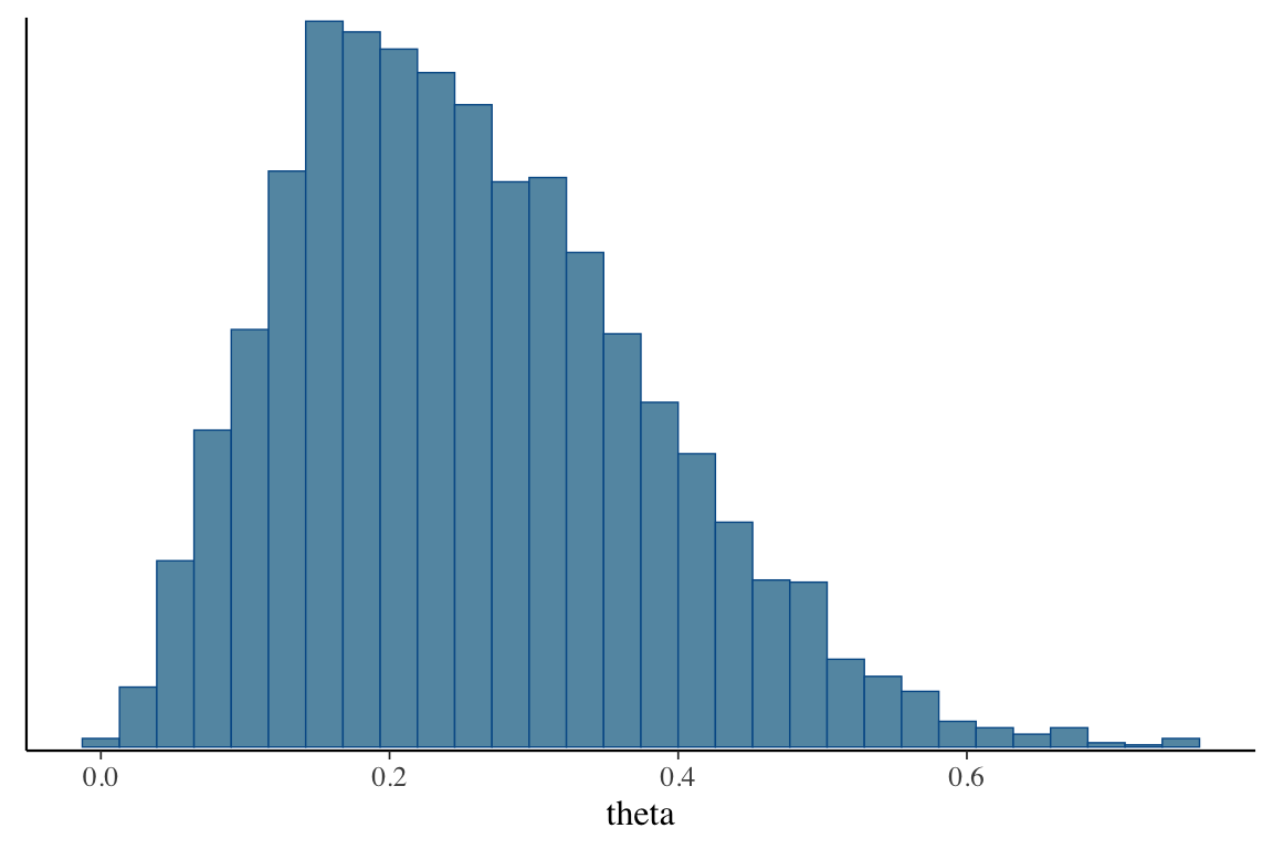
実際には,最初に CmdStanModel オブジェクトを生成し,compile() メソッドを呼び出している.これが compile = TRUE フラッグの存在意義である.↩︎