正規化流

A Blog Entry on Bayesian Computation by an Applied Mathematician

$$

$$

関連ページ

1 概観

正規化流 (NF: Normalizing Flow) とは (Tabak and Vanden-Eijnden, 2010), (Tabak and Turner, 2013) が提案・造語した生成モデリングアプローチである．

ニューラルネットワークとしては画像生成を念頭に置いた密度推定モデルである NICE (Dinh et al., 2015)（のちに Real NVP (Dinh et al., 2017)）が初期のものであり，正則化流を有名にした．

また変分推論のサブルーチンとして正則化流を使えば，効率的な reparametrization trick を可能にするというアイデア (Rezende and Mohamed, 2015) も普及に一役買ったという (Kobyzev et al., 2021)．

アイデアとしては，ニューラルネットワークの一層一層を可逆に設計するという制約を課すのみである．

1.1 原理

1.1.1 基底分布の押し出しとしての生成モデリング

GAN，VAE，拡散モデル など，深層生成モデルは，潜在空間 $\mathcal{Z}$ 上の基底分布 $p(z)dz$ を，パラメータ $w\in \mathcal{W}$ を持つ深層ニューラルネットによる変換 $f_w:\mathcal{Z}\times \mathcal{W}\to \mathcal{X}$ を通じて，押し出し $$p_w(x):=(f_w{)}_{\ast }p(x)$$ により $\mathcal{X}$ 上の分布をモデリングする．

このモデル $\{p_w{\}}_{w\in \mathcal{W}}$ の尤度は解析的に表示できない．そこで，GAN (Goodfellow et al., 2014) は敵対的な学習規則を用いれば，尤度の評価を回避できるというアイデアに基づくものであり，VAE (Kingma and Welling, 2014) は変分下界を通じて尤度を近似するというものであった．

1.1.2 逆変換の利用

正規化流 (normalizing flow / flow-based models) では，拡散モデル に似て，「逆変換」を利用することを考える．

すなわち，$\{f_w\}\subset \mathcal{L}(\mathcal{Z},\mathcal{X})$ が可逆であるように設計するのである．逆関数を $g_w:=f_w^{-1}$ と表すと，$p_w(x)dx$ は $p(z)dz$ の $g_w$ による引き戻しの関係になっているから，変数変換 を通じて， $$p_w(x)=p(g_w(x))|det{J}_{g_w}(x)|\mathrm{a}.\mathrm{e}.$$ が成立する．

すると， $$\log p_w(x)=\log p(g_w(x))+\log |det{J}_{g_w}(x)|$$ を通じて，尤度の評価とパラメータの最尤推定が可能である．

1.2 実装

従って，可逆なニューラルネットワーク $\{f_w\}\subset \mathcal{L}(\mathcal{Z},\mathcal{X})$ を設計することを考える．これは，各層が可逆な変換を定めるようにすることが必要十分である．¹

このとき，行列式 $det:{\mathrm{GL}}_n(\mathbb{R})\to {\mathbb{R}}^{\times }$ は群準同型であるから，$g_w$ のヤコビアンは，各層のヤコビアンの積として得られ，その対数は $$\log |det{J}_{g_w}(x)|=\sum _{i=1}^n\log |det{J}_{g_i}(z_i)|,z_i:=f_i\circ \cdots \circ f_1(z),$$ と得られる．

この条件はたしかにモデルに仮定を置いている．$p(z)dz$ は典型的に正規で，$f_w$ は可逆である．

しかしそれでも，深層ニューラルネットワーク $\{f_w\}$ の表現力は十分高いため，多様な密度のモデリングにも使うことが出来る (Papamakarios et al., 2021)．

1.3 アーキテクチャ

次節 2 で紹介するカップリング流は大変親しみやすい．

その特別な場合として自己回帰流（第 3 節）があり，複雑な成分間の条件付き構造をモデリングできるが，その分高次元データに対する密度評価とサンプリングは遅くなる．

2 カップリング流

2.1 概要

ある可微分同相 $f_{\theta }:{\mathbb{R}}^m\to {\mathbb{R}}^m$ と任意の関数 $\mathrm{\Theta }:{\mathbb{R}}^{n-m}\to {\mathbb{R}}^{n-m}$ について， $$(z^{(1)},z^{(2)})\mapsto (f_{\mathrm{\Theta }(z^{(2)})}(z^{(1)}),z^{(2)})$$ で定まる変換を カップリング層，$f$ をカップリング関数，$\mathrm{\Theta }$ を conditioner という．

(Kingma and Dhariwal, 2018) では，conditioner には ResNet を使っている．

この逆変換は $$(x^{(1)},x^{(2)})\mapsto (f_{\mathrm{\Theta }(x^{(2)})}^{-1}(x^{(1)}),x^{(2)})$$ で与えられる．

加えて，後半の成分 $(-{)}^{(2)}$ には変換を施していないので，カップリング層の Jacobian は $f_{\theta }$ の Jacobian に一致する．

$f_{\theta }$ は各成分が可逆になるように設計することで $f_{\theta }^{-1}$ が計算しやすくされることが多い．

2.2 Real NVP

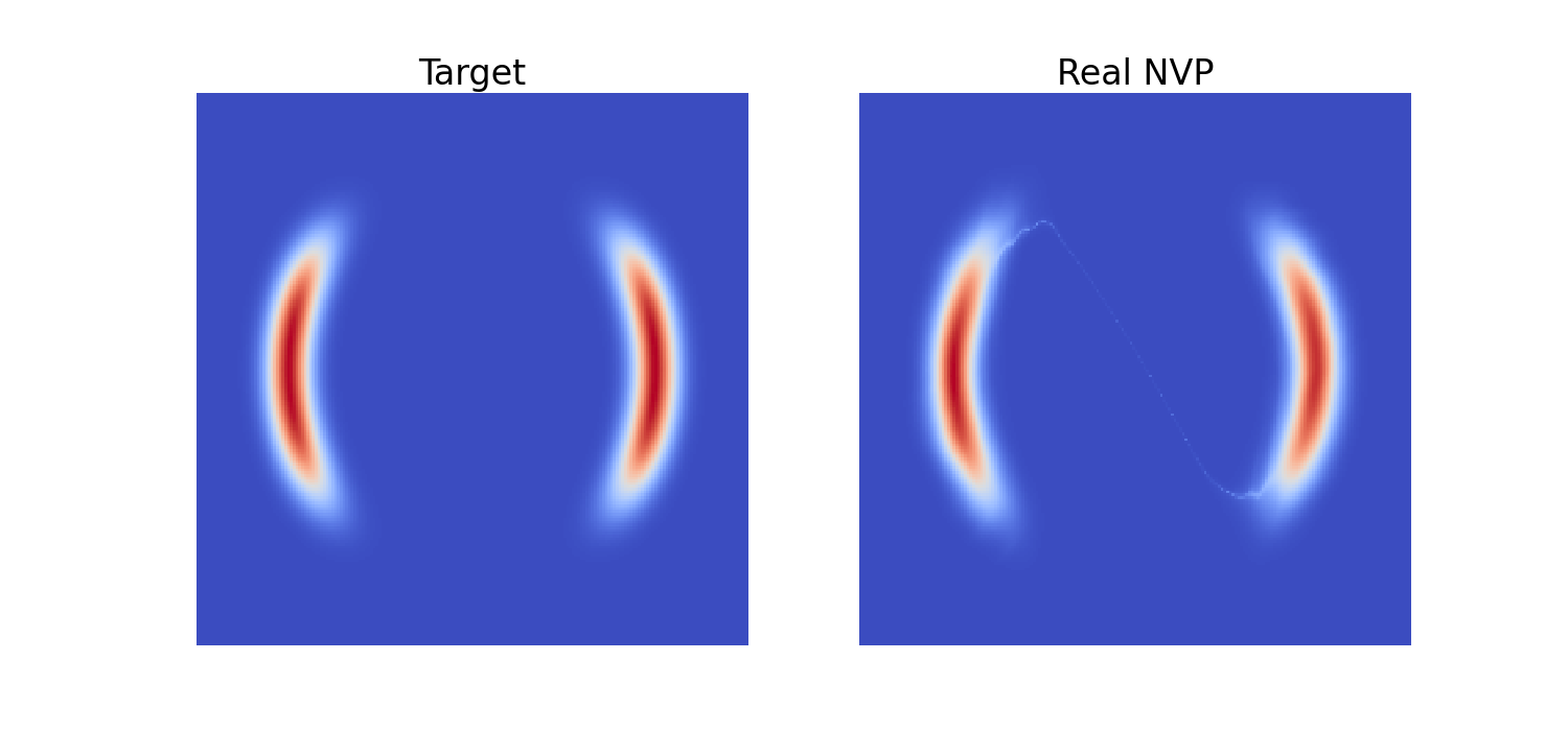
カップリング流を最初に提案したのが NICE (Non-linear Independent Component Estimation) (Dinh et al., 2015) であり，これを画像データに応用したのが (Dinh et al., 2017) の RealNVP (Real-valued Non-Volume-Preserving) である．

NICE では affine カップリング $$f_{\theta }(x)={\theta }_{1}x+{\theta }_2$$ を考えていたが，RealNVP ではさらに $$f_{\mathrm{\Theta }(z^{(2)})}(z^{(1)})=e^{f_{\mathrm{\Theta }(z^{(2)})}^{(1)}}\odot z^{(1)}+f_{\mathrm{\Theta }(z^{(2)})}^{(2)}(z^{(1)}),$$ という形を与えている．ただし $\odot$ はベクトルの成分ごとの積とした．

実際に訓練する変換は $f_{\theta }^{(1)},f_{\theta }^{(2)}$ のみであり，これを可逆に制約するということはなく，実装も簡単になっている．

こうして得たカップリング層を，分割 $z\mapsto (z^{(1)},z^{(2)})$ を取り替えながら（permutation layer と呼ばれる） 32 層重ねるのみで，効率的な密度モデリングができる：

画像をタップしてコードを見る

2.3 GLOW (Kingma and Dhariwal, 2018)

Real NVP では簡単な置換 (permutation) が用いられていたところを，(Kingma and Dhariwal, 2018) では，$1\times 1$ の畳み込みに基づく，一般化されたカップリング・アーキテクチャを提案した．

このことによる計算量の増加は，LU 分解の利用によって回避している．

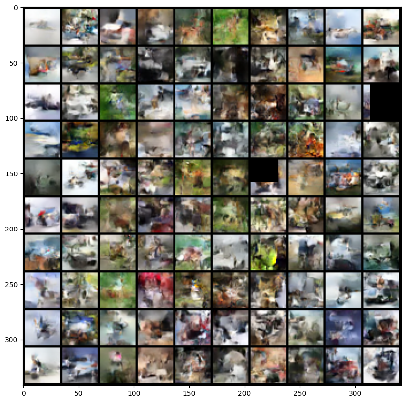
OpenAI release に発表されているように，画像生成タスクに応用された．

3 自己回帰流

3.1 概要

自己回帰流 (autoregressive flow) とは，カップリング流のカップリング関数 $f_{\theta }$ を極限まで押し進めた立場である．

入力 $z\in {\mathbb{R}}^n$ を形式上時系列と見做し，ある可微分関数 $f_{\theta }:\mathbb{R}\to \mathbb{R}$ と任意の関数列 ${\mathrm{\Theta }}_i$ について， $$x_i=f_{{\mathrm{\Theta }}_i(x_{1:i-1})}(z_i)$$ と再帰的に定義していく変換 $z\mapsto x$ を 自己回帰流 という．

この逆は $$z_i=f_{{\mathrm{\Theta }}_i(x_{1:i-1})}^{-1}(x_i)$$ で与えられる．

自己回帰流の Jacobi 行列は上三角行列になるので，Jacobian は効率的に計算できる．

3.2 マスク付き自己回帰流 (MAF)

${\mathrm{\Theta }}_i$ を単一の自己回帰型ニューラルネットワークを用いてモデリングするためには，${\mathrm{\Theta }}_i$ が $x_{1:i-1}$ のみに依存するようにマスク (Germain et al., 2015) をするとよい．

こうすることで $x_1,x_2,\cdots$ と順々に生成する必要はなくなり，並列で計算することができる．（しかし逆の計算は並列化はできない）．

この方法を採用したのが MAF (Masked Autoregressive Flow) (Papamakarios et al., 2017) であった．

MAF では $f$ は affine 関数としている．

3.3 逆自己回帰流 (IAF)

$f$ と $f^{-1}$ を取り替え $$x_i=f_{{\mathrm{\Theta }}_i(z_{1:i-1})}(z_i)$$ としてモデリングする方法を IAF (Inverse Autoregressive Flow) (Kingma et al., 2016) という．

これにより $x_i$ の生成のために $x_1,\cdots ,x_{i-1}$ を先に評価する必要がなく，並列で生成することが可能になり，サンプリングが高速になる．

従って IAF はサンプリング用途に使われるが，その分 MAF より密度評価が遅くなってしまう (Papamakarios et al., 2017)．

3.4 Parallel WaveNet でのサンプリング加速

Parallel WaveNet (Oord et al., 2018) では，WaveNet モデル $p_t$ からのサンプリングを加速させる方法として IAF $p_s$ を用いている．

$p_t$ の密度評価は高速であったため，$\mathrm{KL}(p_s,p_t)$ の値は，$p_t$ の評価と IAF $p_s$ からのサンプリングによって効率的に計算できる．

この KL 乖離度を最適化することで $p_t$ のモデルを $p_s$ に移すことで，サンプルの質を保ちながらサンプリングを加速することに成功した．

4 １変数関数の積によるフロー

4.1 はじめに

カップリング流と自己回帰流はいずれも変換 $f_{\theta }:{\mathbb{R}}^m\to {\mathbb{R}}^m$ に基づいており，次元 $m\le n$ が違うに過ぎない．

この $f_{\theta }$ の表現力を高めることも重要である．

そのためには，1次元の写像 $f_{\theta }^i:\mathbb{R}\to \mathbb{R}$ の積 $f=(f^i)$ としてデザインすることもできる．

このアプローチを element-wise flow ともいう (Kobyzev et al., 2021)．

4.2 スプライン

指定した点 $\{(x_i,y_i)\}$ をなめらかに補間する曲線を一般に スプライン という．

単調関数によって補間すると約束すれば，可逆な変換 $f^i$ を得る．

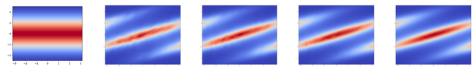
スプラインを，2つの二次関数の商 (rational-quadratic spline) によって補間する方法を提案したのが，Neural Spline Flow (Durkan et al., 2019) である．

この方法では，指定した点 $(x_i,y_i)$ における微分係数が学習すべきパラメータとなる．

例えば von Mises 分布が次のようにモデリングできる：

画像をタップでコードを見る

5 残差フロー

5.1 はじめに

残差接続 $$u\mapsto u+F(u)$$ において，残差ブロック $F$ が縮小写像になるようにすれば，全体として可逆な層となる．

iResNet (Invertible Residual Networks) (Behrmann et al., 2019) では，縮小写像 $F$ のモデリングに CNN を用いた．

この方法のボトルネックは Jacobian の計算にある．愚直に計算すると入力の次元 $d$ に関して $O(d^3)$ の計算量が必要になるため，なんらかの方法で効率化が必要である．

Residual Flow (R. T. Q. Chen et al., 2019) では，Jacobian の推定に Monte Carlo 推定量を用いた．

5.2 Jacobian が計算可能な場合

$J_F$ のランクが低い場合は，$I+J_F$ の形の行列の Jacobian は効率的に計算できる．

Planar flow (Rezende and Mohamed, 2015) では隠れ素子数１の残差接続層を用いたものである： $$f(u)=u+v\sigma (w^{\mathrm{\top }}u+b).$$ この設定では Jacobian が次のように計算できる： $$det{J}_f(u)=1+w^{\mathrm{\top }}v{\sigma }^{\prime }(w^{\mathrm{\top }}u+b).$$

ただし非線型な活性化関数 $\sigma$ は全単射になるように選ぶ必要がある．

証明

この Jacobian を導出する際には，次の Matrix determinant lemma を用いる．

$$det(A+u{v}^{\mathrm{\top }})=det(A)(1+v^{\mathrm{\top }}{A}^{-1}u).$$

これは行列式の多重歪線型性を用いて簡単に示すことができる．

Planar flow の欠点は逆の計算が難しい点であり，現在広く使われるわけではない (Kobyzev et al., 2021)．

他に，circular flow (Rezende and Mohamed, 2015) や Sylvester flow (Berg et al., 2019) も同様な解析的な Jacobian の表示を与えるアーキテクチャである．

Sylvester flow (Berg et al., 2019) は $\sigma$ を多次元化したものである．この際の Jacobian は Sylvester の行列式の補題 により導かれることから名前がついた： $$det(I_n+AB)=det(I_m+BA).$$

5.3 Jacobian を推定する方法

仮に変換 $F$ に制約を課さずとも，Jacobian は $$\log |det(I+J_F)|=\sum _{k=1}^{\mathrm{\infty }}\frac{(-1{)}^{k+1}}{k}\mathrm{Tr}(J_F^k)$$ を通じて，$\mathrm{Tr}(J_F)$ が (Skilling, 1989)-(Hutchinson, 1990) の跡推定量 により，その無限和が Russian-roulette 推定量により不偏推定できる (R. T. Q. Chen et al., 2019)．

Russian-roulette 推定量では，無限和を最初の $N$ 項のみの有限和で近似するとバイアスが入るので，$N$ を確率変数とすることで不偏推定が達成される．

6 応用

6.1 変分推論のサブルーチンとして

変分推論における $E$-ステップ（変分分布について期待値を取るステップ）などにおいて，複雑な分布からのサンプラーとしても用いられる (Gao et al., 2020)．

この使い方を初めて提唱し，フローベースのアプローチを有名にしたのが (Rezende and Mohamed, 2015) であった．

このような変分ベイズ推論，特にベイズ深層学習に向けたフローベースモデルが盛んに提案されている．

Householder flow (Tomczak and Welling, 2017) は VAE の改良のために考えられたものである．直交行列で表現できる層を，直行行列の Householder 行列の積として表現することで学習することを目指す．

他にも IAF (Kingma et al., 2016), 乗法的正規化流 (Louizos and Welling, 2017), Sylvester flow (Berg et al., 2019) など．

6.2 ベイズ計算

Neural Importance Sampling (Müller et al., 2019) とは，困難な分布からの重点サンプリングの際に，提案分布を正規化流で近似する方法である．この際に $f_{\theta }(x)$ にはスプラインを用いている．

Boltzmann Generator (Noé et al., 2019) は名前の通り，多体系の平衡分布から正規化流でサンプリングをするという手法である．

(Hoffman et al., 2019) は IAF を用いて目標分布を学習し，学習された密度 $q$ で変換後の分布から MCMC サンプリングをすることで効率がはるかに改善することを報告した．実際，フローによる変換を受けた後は対象分布は正規分布に近くなることから，MCMC サンプリングを減速させる要因の多くが消滅していることが期待される．

6.3 密度推定

目標の分布 $p_w$ を Guass 分布 $p$ からの写像 $(f_w{)}_{\ast }p$ として捉える発想は，まずなんといっても密度推定に用いられた (S. Chen and Gopinath, 2000)．この時点では Gaussianization と呼ばれていた．

この $f_w$ のモデリングにニューラルネットワークを用いるという発想は (Rippel and Adams, 2013) の Deep Density Model 以来であるようだ．

その後同様の発想は非線型独立成分分析 (Dinh et al., 2015)，引き続き密度推定 (Dinh et al., 2017) に用いられた．

現在は MAF 3.2 の性能が圧倒的である．

6.4 表現学習

通常の VAE などは，あくまで $p(x|z)$ を学習する形をとるが，正規化流を用いて結合分布 $p(x,z)$ を学習することで，双方を対等にモデリングすることができる．

これを flow-based hybrid model (Nalisnick et al., 2019) という．これは予測と生成のタスクでも良い性能を見せるが，分布外検知などの応用も示唆している．

異常検知 (Zhang et al., 2020)，不確実性定量化 (Charpentier et al., 2020) のような種々の下流タスクに用いられた場合は，VAE など NN を２つ用いる手法よりもモデルが軽量で，順方向での１度の使用で足りるなどの美点があるという．

6.5 生成

画像生成への応用が多い：GLOW (Kingma and Dhariwal, 2018) (OpenAI release), 残差フロー (R. T. Q. Chen et al., 2019) など．

動画に対する応用も提案されている：VideoFlow (Kumar et al., 2020)．

言語に対する応用もある (Tran et al., 2019)．言語は離散データであることが難点であるが，潜在空間上でフローを使うことも提案されている (Ziegler and Rush, 2019)．

6.6 蒸留

純粋な生成モデリングの他に，IAF 3.3 は (Oord et al., 2018) において音声生成モデルの蒸留に用いられた．

WaveFLOW (Prenger et al., 2018), FloWaveNet (Kim et al., 2019) などもカップリング層を取り入れて WaveNet の高速化に成功している．

6.7 SBI

モデルの尤度は隠されており，入力 $\theta$ に対して，$p(x|\theta )$ からのサンプルのみが利用可能であるとする．このような状況でベイズ推論を行う問題を simulation-based inference (SBI) という．

これはデータの分布のサンプルから学習して，似たようなデータを増やすという生成モデルのタスクに似ており，正則化流との相性が極めて良い (Cranmer et al., 2020)．

この際，任意の分布 $p(\theta )$ に対して，結合分布 $$p(x,\theta )=p(x|\theta )p(\theta )$$ を，シミュレータから得られるサンプルのみからフローベースモデルにより学習してしまうことで，ベイズ償却推論が可能になる (Papamakarios et al., 2019)．

この方法はさらに，事後分布推定に特化することで，SMC-ABC などの従来の近似ベイズ計算技法の性能を超えていくようである (Greenberg et al., 2019)．

BayesFlow (Radev et al., 2022) は観測データからモデルパラメータへのフローを，償却推論によって学習する．一度このフローが学習されれば，新たなデータの到着に対しても極めて安価な限界費用で推論を更新できる．

7 文献

Janosh Riebesell のリポジトリ awesome-normalizing-flows に実装がまとめられている．

(Murphy, 2023) 第23章は入門に良い．詳細はサーベイ (Kobyzev et al., 2021), (Papamakarios et al., 2021) に譲られている．

(S. Chen and Gopinath, 2000) の時点では同様のアイデアは Gaussianization と呼ばれていた．

(Tabak and Vanden-Eijnden, 2010), (Tabak and Turner, 2013) が (S. Chen and Gopinath, 2000) のアイデアを推し進めて，確率測度のフローによる押し出しとしての正規化流の提案と命名を行った．このフローの学習は最尤推定によって行なっていた．

References

Behrmann, J., Grathwohl, W., Chen, R. T. Q., Duvenaud, D., and Jacobsen, J.-H. (2019). Invertible residual networks. In K. Chaudhuri and R. Salakhutdinov, editors, Proceedings of the 36th international conference on machine learning,Vol. 97, pages 573–582. PMLR.

Berg, R. van den, Hasenclever, L., Tomczak, J. M., and Welling, M. (2019). Sylvester normalizing flows for variational inference. In Conference on uncertainty in artificial intelligence,Vol. 34, pages 393–402.

Charpentier, B., Zügner, D., and Günnemann, S. (2020). Posterior network: Uncertainty estimation without OOD samples via density-based pseudo-counts. In H. Larochelle, M. Ranzato, R. Hadsell, M. F. Balcan, and H. Lin, editors, Advances in neural information processing systems,Vol. 33, pages 1356–1367. Curran Associates, Inc.

Chen, R. T. Q., Behrmann, J., Duvenaud, D. K., and Jacobsen, J.-H. (2019). Residual flows for invertible generative modeling. In H. Wallach, H. Larochelle, A. Beygelzimer, F. dAlché-Buc, E. Fox, and R. Garnett, editors, Advances in neural information processing systems,Vol. 32. Curran Associates, Inc.

Chen, S., and Gopinath, R. (2000). Gaussianization. In T. Leen, T. Dietterich, and V. Tresp, editors, Advances in neural information processing systems,Vol. 13. MIT Press.

Cranmer, K., Brehmer, J., and Louppe, G. (2020). The frontier of simulation-based inference. Proceedings of the National Academy of Sciences, 117(48), 30055–30062.

Dinh, L., Krueger, D., and Bengio, Y. (2015). NICE: Non-linear independent components estimation. In International conference on learning representations. poster.

Dinh, L., Sohl-Dickstein, J., and Bengio, S. (2017). Density estimation using real NVP. In International conference on learning representations.

Durkan, C., Bekasov, A., Murray, I., and Papamakarios, G. (2019). Neural spline flows. In H. Wallach, H. Larochelle, A. Beygelzimer, F. dAlché-Buc, E. Fox, and R. Garnett, editors, Advances in neural information processing systems,Vol. 32. Curran Associates, Inc.

Gao, R., Nijkamp, E., Kingma, D. P., Xu, Z., Dai, A. M., and Wu, Y. N. (2020). Flow contrastive estimation of energy-based models. In Proceedings of the IEEE/CVF conference on computer vision and pattern recognition (CVPR).

Germain, M., Gregor, K., Murray, I., and Larochelle, H. (2015). MADE: Masked Autoencoder for Distribution Estimation. In F. Bach and D. Blei, editors, Proceedings of the 32nd international conference on machine learning,Vol. 37, pages 881–889. Lille, France: PMLR.

Goodfellow, I., Pouget-Abadie, J., Mirza, M., Xu, B., Warde-Farley, D., Ozair, S., … Bengio, Y. (2014). Generative adversarial nets. In Advances in neural information processing systems,Vol. 27, pages 1–9.

Greenberg, D., Nonnenmacher, M., and Macke, J. (2019). Automatic posterior transformation for likelihood-free inference. In K. Chaudhuri and R. Salakhutdinov, editors, Proceedings of the 36th international conference on machine learning,Vol. 97, pages 2404–2414. PMLR.

Hoffman, M., Sountsov, P., Dillon, J. V., Langmore, I., Tran, D., and Vasudevan, S. (2019). NeuTra-lizing bad geometry in hamiltonian monte carlo using neural transport. In Symposium on advances in approximate bayesian inference.

Hutchinson, M. F. (1990). A Stochastic Estimator of the Trace of the Influence Matrix for Laplacian Smoothing Splines. Communications in Statistics - Simulation and Computation, 19(2), 433–450. doi: 10.1080/03610919008812866.

Kim, S., Lee, S.-G., Song, J., Kim, J., and Yoon, S. (2019). FloWaveNet : A generative flow for raw audio. In K. Chaudhuri and R. Salakhutdinov, editors, Proceedings of the 36th international conference on machine learning,Vol. 97, pages 3370–3378. PMLR.

Kingma, D. P., and Dhariwal, P. (2018). Glow: Generative flow with invertible 1x1 convolutions. In S. Bengio, H. Wallach, H. Larochelle, K. Grauman, N. Cesa-Bianchi, and R. Garnett, editors, Advances in neural information processing systems,Vol. 31. Curran Associates, Inc.

Kingma, D. P., Salimans, T., Jozefowicz, R., Chen, X., Sutskever, I., and Welling, M. (2016). Improved variational inference with inverse autoregressive flow. In D. Lee, M. Sugiyama, U. Luxburg, I. Guyon, and R. Garnett, editors, Advances in neural information processing systems,Vol. 29. Curran Associates, Inc.

Kingma, D. P., and Welling, M. (2014). Auto-encoding variational bayes. In International conference on learning representations,Vol. 2.

Kobyzev, I., Prince, S. D., and Brubaker, M. A. (2021). Normalizing flows: An introduction and review of current methods. IEEE Transactions on Pattern Analysis &Amp; Machine Intelligence, 43(11), 3964–3979.

Kumar, M., Babaeizadeh, M., Erhan, D., Finn, C., Levine, S., Dinh, L., and Kingma, D. (2020). VideoFlow: A conditional flow-based model for stochastic video generation. In International conference on learning representations.

Louizos, C., and Welling, M. (2017). Multiplicative normalizing flows for variational bayesian neural networks. In Proceedings of the 34th international conference on machine learning - volume 70, pages 2218–2227. Sydney, NSW, Australia: JMLR.org.

Müller, T., Mcwilliams, B., Rousselle, F., Gross, M., and Novák, J. (2019). Neural importance sampling. ACM Trans. Graph., 38(5).

Murphy, K. P. (2023). Probabilistic machine learning: Advanced topics. MIT Press.

Nalisnick, E., Matsukawa, A., Teh, Y. W., Gorur, D., and Lakshminarayanan, B. (2019). Hybrid models with deep and invertible features. In International conference on machine learning.

Noé, F., Olsson, S., Köhler, J., and Wu, H. (2019). Boltzmann generators: Sampling equilibrium states of many-body systems with deep learning. Science, 365(6457), eaaw1147.

Oord, A. van den, Li, Y., Babuschkin, I., Simonyan, K., Vinyals, O., Kavukcuoglu, K., … Hassabis, D. (2018). Parallel WaveNet: Fast high-fidelity speech synthesis. In J. Dy and A. Krause, editors, Proceedings of the 35th international conference on machine learning,Vol. 80, pages 3918–3926. PMLR.

Papamakarios, G., Nalisnick, E., Rezende, D. J., Mohamed, S., and Lakshminarayanan, B. (2021). Normalizing flows for probabilistic modeling and inference. J. Mach. Learn. Res., 22(1).

Papamakarios, G., Pavlakou, T., and Murray, I. (2017). Masked autoregressive flow for density estimation. In I. Guyon, U. V. Luxburg, S. Bengio, H. Wallach, R. Fergus, S. Vishwanathan, and R. Garnett, editors, Advances in neural information processing systems,Vol. 30. Curran Associates, Inc.

Papamakarios, G., Sterratt, D., and Murray, I. (2019). Sequential neural likelihood: Fast likelihood-free inference with autoregressive flows. In K. Chaudhuri and M. Sugiyama, editors, Proceedings of the twenty-second international conference on artificial intelligence and statistics,Vol. 89, pages 837–848. PMLR.

Prenger, R., Valle, R., and Catanzaro, B. (2018). WaveGlow: A flow-based generative network for speech synthesis.

Radev, S. T., Mertens, U. K., Voss, A., Ardizzone, L., and Köthe, U. (2022). BayesFlow: Learning complex stochastic models with invertible neural networks. IEEE Transactions on Neural Networks and Learning Systems, 33(4), 1452–1466.

Rezende, D., and Mohamed, S. (2015). Variational inference with normalizing flows. In F. Bach and D. Blei, editors, Proceedings of the 32nd international conference on machine learning,Vol. 37, pages 1530–1538. Lille, France: PMLR.

Rippel, O., and Adams, R. P. (2013). High-dimensional probability estimation with deep density models.

Skilling, J. (1989). The eigenvalues of mega-dimensional matrices. In J. Skilling, editor, Maximum entropy and bayesian methods: Cambridge, england, 1988, pages 455–466. Dordrecht: Springer Netherlands.

Tabak, E. G., and Turner, C. V. (2013). A family of nonparametric density estimation algorithms. Communications on Pure and Applied Mathematics, 66(2), 145–164.

Tabak, E. G., and Vanden-Eijnden, E. (2010). Density estimation by dual ascent of the log-likelihood. Communications in Mathematical Sciences, 8(1), 217–233.

Tomczak, J. M., and Welling, M. (2017). Improving variational auto-encoders using householder flow.

Tran, D., Vafa, K., Agrawal, K., Dinh, L., and Poole, B. (2019). Discrete flows: Invertible generative models of discrete data. In H. Wallach, H. Larochelle, A. Beygelzimer, F. dAlché-Buc, E. Fox, and R. Garnett, editors, Advances in neural information processing systems,Vol. 32. Curran Associates, Inc.

Zhang, H., Li, A., Guo, J., and Guo, Y. (2020). Hybrid models for open set recognition. In A. Vedaldi, H. Bischof, T. Brox, and J.-M. Frahm, editors, Computer vision – ECCV 2020, pages 102–117. Cham: Springer International Publishing.

Ziegler, Z., and Rush, A. (2019). Latent normalizing flows for discrete sequences. In K. Chaudhuri and R. Salakhutdinov, editors, Proceedings of the 36th international conference on machine learning,Vol. 97, pages 7673–7682. PMLR.

Footnotes

1. この考え方は，VAE ではデコーダーをエンコーダーを用いていたものを，１つの可逆な NN で済ましているようにみなせる．