Masked Diffusion Models

A Blog Entry on Bayesian Computation by an Applied Mathematician

$$

$$

1 Introduction

1.1 A Time-Agnostic Learning Framework

The absorbing process, a.k.a. masked diffusion, has a unique characteristic as a forward process in a discrete denoising diffusion model; it offers a time-agnostic learning to unmask training framework.

When the state space is \(E^d\) where \(E=\{0,\cdots,K-1\}\) is finite, a current practice is to learn a neural network \(p_\theta\) based on a loss given by \[ \mathcal{L}(\theta):=\int^1_0\frac{\dot{\alpha}_t}{1-\alpha_t}\operatorname{E}\left[\sum_{i=1}^d\log p_\theta(X_0^i|X_t)\right]\,dt, \tag{1}\] where \(\alpha_t\) is a noising schedule, determining the convergence speed of the forward process.¹

The expectation in (1) is exactly a cross-entropy loss. Therefore, the loss (1) can be understood as a weighted cross-entropy loss, weighted by the noising schedule \(\alpha_t\).

Note that \(p_\theta\) predicts the true state \(x_0\), based on the current state \(x_t\), some components of which might be masked. Hence we called this framework learning to unmask.

Note also that \(p_\theta\) doesn’t take \(t\) as an argument (Shi et al., 2024), (Ou et al., 2025), which we call the time-agnostic property, following (Zheng et al., 2025).

1.2 Choice of \(\alpha_t\)

This ‘learning to unmask’ task might be very hard when \(t\) is near \(1\), since most of the \(x_t^i\)’s are still masked.

For instance, if we choose a linear schedule \[ \alpha_t=1-t\qquad(t\in[0,1]) \] the scaler \(\frac{\dot{\alpha}_t}{1-\alpha_t}=-t^{-1}\) before the expectation in (1) puts less weight on large \(t\approx1\), while puts much more weight on small \(t\approx0\), where most of the \(x_t^i\)’s should be already unmasked.

Hence, selecting the schedule \(\alpha_t\) to make learning easier can be very effective, for example by reducing the variance of gradient estimator in a SGD algorithm. Actually, this is a part of the technique how (Arriola et al., 2025) achieved their remarkable empirical results.

This flexibility of \(\alpha_t\) is why the loss (1) is considered as a potential competitor against the current dominant autoregressive models. In fact, one work (Chao et al., 2025), still under review, claimed their masked diffusion model surpassed the autoregressive model on the task of language modeling, achieving an evaluation perplexity of 15.36 on the OpenWebText dataset.²

We briefly discuss their trick and related promising techniques to improve the model, before programming toy examples in Section 2 and Section 3 to deepen our understanding in absorbing forward process.

1.3 A Gibbs Sampler Take

One problem about the loss (1) is that \(p_\theta\) predicts the unmasked complete sequence in a product form: \[ p_\theta(x_0|x_t)=\prod_{i=1}^d p_\theta(x_0^i|x_t). \]

This should cause no problem when we unmask one component at a time, since it will be a form of ancestral sampling based on disintegration property.

However, when unmasking two or more components simultaneously, for example when the number of steps is less than \(d\), the product form assumption will simply introduce a bias, as the data distribution is by no means of product form on \(E^d\).

Here, to recover correctness asymptotically, analogy with Gibbs sampling becomes very important.

For example, predictor-corrector technique can be readily employed to mitigate this bias, as discussed in (Lezama et al., 2023), (S. Zhao et al., 2024), (L. Zhao et al., 2024), (Gat et al., 2024), (Wang et al., 2025).

We demonstrate this strategy in Section 3.5.

1.4 Intermediate States

As we mentioned earlier, unmasking can be a very hard task, as closely investigated in (Kim et al., 2025, sec. 3).

To alleviate this problem, (Chao et al., 2025) introduced intermediate states by re-encoding the token in a base-\(2\) encoding, such as \[ 5\mapsto 101. \] The right-hand side needs three steps to be completely unmasked, while the left-hand side only needs one jump.

Therefore, unmasking can be easier to learn, compared to the original token encoding.

However, this is not the only advantage of intermediate states. (Chao et al., 2025) were able to construct a full predictor \(p_\theta\) without the product form assumption on each token.

This approach might act as a block Gibbs sampler and make the convergence faster, as we will discuss later in Section 3.6.

1.5 State-Dependent Rate

As a function of \(t\mapsto\alpha_t\), different choices for \(\alpha_t\) seem to make little impact on the total performance of the model, as we observe in our toy example in Section 2.4.

However, if we allow \(\alpha_t\) to depend on the state as in (Shi et al., 2024, sec. 6), I believe the masked diffusion model will start to show its real potential over currently dominant autoregressive framework.

A problem arises when one tries to learn \(\alpha_t\) at the same time, for example, by including a corresponding term into the loss (1). This will lead to amplified variances of the gradient estimates and unstable training, as reported in (Shi et al., 2024) and (Arriola et al., 2025).

The idea of exploiting state-dependent rate is already very common in sampling time (Peng et al., 2025), (Liu et al., 2025), (Kim et al., 2025), (Rout et al., 2025), determining which token to unmask next during the backward sampling, a bit like Monte Carlo tree search in reinforcement learning.

2 Demo

To demonstrate what an absorbing process does, we carry out generation from a toy data distribution \(\pi_{\text{data}}\) on \(5=\{0,1,2,3,4\}\), by running an exact reverse kernel of the absorbing (masked) forward process.

Therefore, no neural network training will be involved. A 2d example, which is much more interesting, in Section 3 will basically process in parallel.

2.1 Setup

import numpy as np
import matplotlib.pyplot as plt

rng = np.random.default_rng(42)

p_data = np.array([0.40, 0.30, 0.18, 0.10, 0.02], dtype=float)

We will represent the MASK as \(-1\). The state space is then \(E:=5 \cup \{-1\}\).

MASK = -1

An important design choice in the forward process is the noising schedule \(\alpha_t\), which can be interpreted as survival probability and satisfy the following relatioship with the jump intensity \(\beta_t\): \[ \alpha_t=\exp\left(-\int^t_0\beta_s\,ds\right),\qquad t\in[0,1]. \]

Let us keep it simple and set \(\alpha_t=t\). To achive this, we need to set \[ \beta_t=\frac{1}{1-t},\qquad t\in[0,1), \] which is clearly diverging as \(t\to1\). This is to ensure the process to converge in finite time.

T = 10  # number of steps
alpha = np.linspace(1.00, 0.00, T+1)

2.2 The Backward Transition Kernel

In this setting, the backward transition kernel \(p(x_{t-1} | x_t)\) satisfies \[ \operatorname{P}[X_{t-1}=-1|X_t=-1]=\frac{1 - \alpha_{t-1}}{1 - \alpha_t}. \] In the other cases, the unmasked values \(x_{t-1}\) should be determined according to \(\pi_{\text{data}}\), which is unavailable in a real setting, of course.

p_unmask = (alpha[:-1] - alpha[1:]) / (1.0 - alpha[1:])  # length T

def reverse_sample(num_samples: int, p_unmask: np.ndarray):
    """
    Start from x_T = MASK for all samples, apply the exact reverse transitions down to t=0.
    Returns x_0 samples in 5 = {0,1,...,4}.
    """
    x_t = np.full(num_samples, MASK, dtype=int)
    hist = np.empty((T+1, num_samples), dtype=int)
    hist[0] = x_t.copy()
    for t in range(T, 0, -1):
        idx_mask = np.where(x_t == MASK)[0]  # masked indices
        if idx_mask.size > 0:
            u = rng.random(idx_mask.size)
            unmask_now = idx_mask[u < p_unmask[t-1]]  # indices that are going to be unmasked
            if unmask_now.size > 0:
                cats = rng.choice(5, size=unmask_now.size, p=p_data)
                x_t[unmask_now] = cats
        hist[T-t+1] = x_t.copy()

    # At t=0, all remaining MASKs (if any) must have already unmasked earlier with probability 1,
    # but numerically we ensure no MASK remains:
    assert np.all(x_t != MASK), "Some samples remained MASK at t=0, which should not happen."
    return x_t, hist

2.2.1 A Note on Alternative Sampling Strategies

Note that we need not to obey this exact backward transition kernel to sample from the data distribution.

For example, remasking (Lezama et al., 2023), (S. Zhao et al., 2024), (Gat et al., 2024), (Wang et al., 2025), a form of predictor-corrector sampling, can be incorporated to improve sample quality, mitigating numerical errors, as we will see in Section 3.5.

Recently, sampling time path planning (Peng et al., 2025), (Liu et al., 2025), (Kim et al., 2025), (Rout et al., 2025) has been proposed to improve sample quality and model log-likelihood, which lay out of the scope of this post.

2.3 Honest Sampling

N = 100_000  # size of sample to get
x0_samples, hist = reverse_sample(N, p_unmask)

We first make sure our implementation is correct by checking the empirical distribution of the samples generated agrees with the true distribution.

counts = np.bincount(x0_samples, minlength=5).astype(float)
p_emp = counts / counts.sum()

print("Toy data marginal p_data:", p_data.round(4))
print("Empirical p after reverse sampling:", p_emp.round(4))

# ---------- Bar chart: p_data vs empirical ----------
xs = np.arange(5)
width = 0.4
plt.figure(figsize=(6,3))
plt.bar(xs - width/2, p_data, width=width, label="true p_data")
plt.bar(xs + width/2, p_emp, width=width, label="empirical (reverse)")
plt.title("Reverse samples match the data marginal")
plt.xlabel("category id")
plt.ylabel("probability")
plt.legend()
plt.tight_layout()
plt.show()

Toy data marginal p_data: [0.4  0.3  0.18 0.1  0.02]
Empirical p after reverse sampling: [0.3979 0.3002 0.1828 0.0992 0.0198]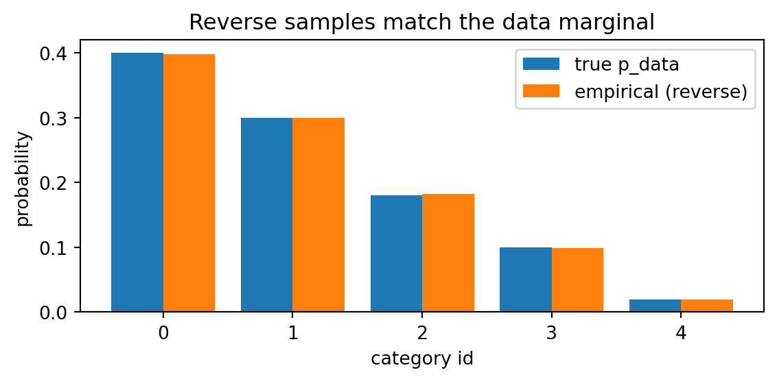

Perfect! Making sure everything is working, we plot 1000 sample paths from the reverse process.

n_samples_to_plot = min(1000, hist.shape[1])
plt.figure()

for i in range(n_samples_to_plot):
    plt.plot(range(hist.shape[0]), hist[:, i], alpha=0.5, linewidth=0.8)

plt.xlabel('Time step')
plt.ylabel('State')
plt.title(f'Sample trajectories (first {n_samples_to_plot} samples)')
plt.grid(True, alpha=0.3)
plt.show()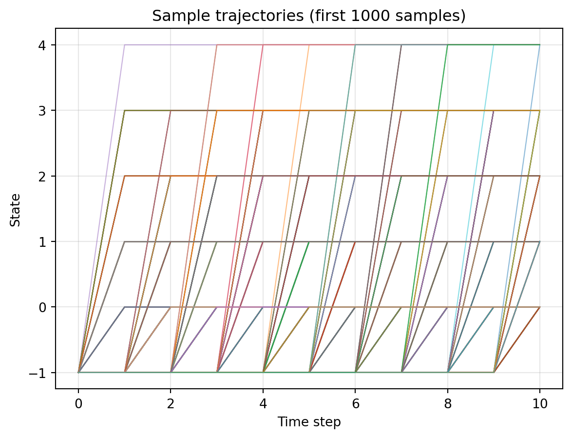

We see a relatively equal number of jumps per step:

jump_counts = np.zeros(T)
for i in range(10):
    jump_counts[i] = sum(hist[i] != hist[i+1])
print(jump_counts)

[ 9916. 10017. 10001. 10143. 10062. 10195.  9815. 10005.  9859.  9987.]

This is because we set \(\alpha_t=1-t\) to be linear.

# ---------- Plot schedule α_t (survival probability) ----------
plt.figure(figsize=(5,3))
plt.plot(range(T+1), alpha, marker="o")
plt.title(r"Survival probability $\alpha_t$")
plt.xlabel("t")
plt.ylabel(r"$\alpha_t$")
plt.tight_layout()
plt.show()

2.4 Choice of \(\alpha_t\)

\(\alpha_t\) controls the convergence rate of the forward process.

We change \(\alpha_t\) to see the impact on the sampling accuracy. (There should be no influence as long as the exact backward kernel is used.)

Let us change \(\alpha_t\) to be an exponential schedule:

alpha_exp = np.exp(np.linspace(0.00, -10.00, T+1))
p_unmask_exp = (alpha_exp[:-1] - alpha_exp[1:]) / (1.0 - alpha_exp[1:])

plt.figure(figsize=(5,3))
plt.plot(range(T+1), alpha_exp, marker="o")
plt.title(r"Survival probability $\alpha_t$")
plt.xlabel("t")
plt.ylabel(r"$\alpha_t$")
plt.tight_layout()
plt.show()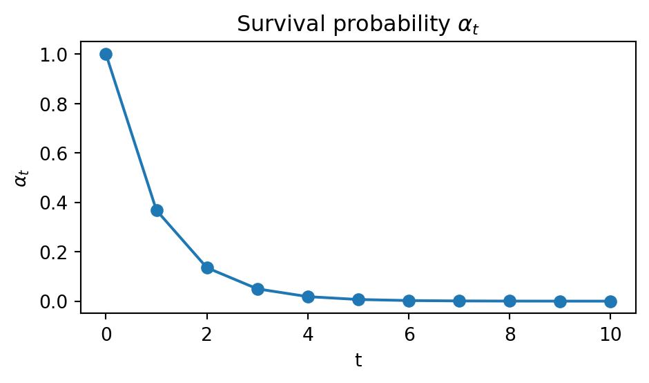

In this way, most of the unmasking events should occur in the very last step of the reverse process.

x0_exp, hist_exp = reverse_sample(N, p_unmask_exp)

n_samples_to_plot = min(1000, hist_exp.shape[1])
plt.figure()

for i in range(n_samples_to_plot):
    plt.plot(range(hist_exp.shape[0]), hist_exp[:, i], alpha=0.5, linewidth=0.8)

plt.xlabel('Time step')
plt.ylabel('State')
plt.title(f'Sample trajectories (first {n_samples_to_plot} samples)')
plt.grid(True, alpha=0.3)
plt.show()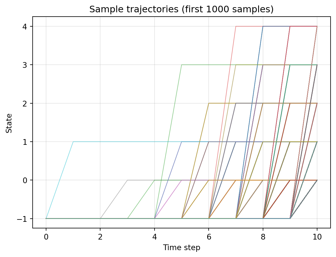

We see many jumps happen in the latter half.

Practically speaking, this is certainly not what we want.

We spend almost half of the computational time (up to the 6th step) in simulating the phantom jumps which just do not happen. The same concern was raised by (Chao et al., 2025).

However, the accuracy is same, as the exact kernel is used to simulate, if the computational cost might be different.

def calc_l1_kl(x0_samples, split = 10):
    chunks = np.array_split(x0_samples, split)
    counts = np.array([np.bincount(chunk, minlength=5).astype(float) for chunk in chunks])

    p_emp = counts / counts.sum(axis=1)[0]
    l1 = np.abs(p_emp - p_data).sum(axis=1).mean()
    l1_var = np.abs(p_emp - p_data).sum(axis=1).var()
    kl = (np.where(p_emp > 0, p_emp * np.log(p_emp / p_data), 0)).sum(axis=1).mean()
    kl_var = (np.where(p_emp > 0, p_emp * np.log(p_emp / p_data), 0)).sum(axis=1).var()
    return l1, l1_var, kl, kl_var

l1, l1_var, kl, kl_var = calc_l1_kl(x0_samples)
print("Linear Schedule: L1 distance:", round(l1, 6), " ± ", round(l1_var, 6), "   KL(p_emp || p_data):", round(kl, 6), " ± ", round(kl_var, 6))

l1_exp, l1_exp_var, kl_exp, kl_exp_var = calc_l1_kl(x0_exp)
print("Exponential Schedule: L1 distance:", round(l1_exp, 6), " ± ", round(l1_exp_var, 6), "   KL(p_emp || p_data):", round(kl_exp, 6), " ± ", round(kl_exp_var, 6))

Linear Schedule: L1 distance: 0.0147  ±  3e-05    KL(p_emp || p_data): 0.000196  ±  0.0
Exponential Schedule: L1 distance: 0.0148  ±  4.9e-05    KL(p_emp || p_data): 0.000232  ±  0.0

3 2D Example

3.1 Setup

We consider a highly correlated distribution, whose support is degenerated on the diagonal element on \(5^2\).

K = 5
MASK = -1

# Base marginal for a single site
p_single = np.array([0.40, 0.30, 0.18, 0.10, 0.02], dtype=float)
p_single /= p_single.sum()

# Build correlated joint with same-parity constraint
W = np.zeros((K, K), dtype=float)
for i in range(K):
    for j in range(K):
        if (i % 2) == (j % 2):
            W[i, j] = p_single[i] * p_single[j]
pi_joint = W / W.sum()
pi_x = pi_joint.sum(axis=1)
pi_y = pi_joint.sum(axis=0)

# Conditionals
cond_x_given_y = np.zeros((K, K), dtype=float)  # [j, i]
cond_y_given_x = np.zeros((K, K), dtype=float)  # [i, j]
for j in range(K):
    col = pi_joint[:, j]; s = col.sum()
    if s > 0:
        cond_x_given_y[j, :] = col / s
for i in range(K):
    row = pi_joint[i, :]; s = row.sum()
    if s > 0:
        cond_y_given_x[i, :] = row / s

fig = plt.figure(figsize=(8, 3.4))

# Heatmap
ax1 = plt.subplot(1, 2, 1)
im = ax1.imshow(pi_joint, cmap='viridis', aspect='equal')
ax1.set_xlabel('Y')
ax1.set_ylabel('X')
ax1.set_title('Joint Probability Distribution (Heatmap)')
ax1.set_xticks(range(K))
ax1.set_yticks(range(K))

# Value annotation
for i in range(K):
    for j in range(K):
        ax1.text(j, i, f'{pi_joint[i, j]:.3f}', 
                ha='center', va='center', color='white', fontsize=8)

plt.colorbar(im, ax=ax1)

# 3D bar plot
ax2 = plt.subplot(1, 2, 2, projection='3d')
x = np.arange(K)
y = np.arange(K)
X, Y = np.meshgrid(x, y)
Z = pi_joint

ax2.bar3d(X.ravel(), Y.ravel(), np.zeros_like(Z.ravel()), 
         0.8, 0.8, Z.ravel(), alpha=0.8, cmap='viridis')

ax2.set_xlabel('Y')
ax2.set_ylabel('X')
ax2.set_zlabel('Probability')
ax2.set_title('Joint Probability Distribution (3D)')
ax2.set_xticks(x)
ax2.set_yticks(y)

plt.tight_layout()
plt.show()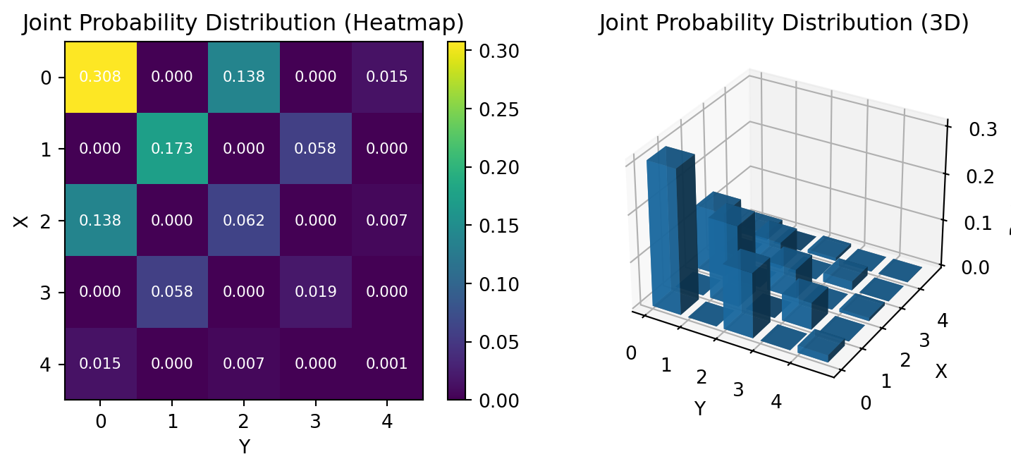

3.2 The Backward Transition Kernel

We will first consider, again, linear schedule:

T = 10
alpha = np.linspace(1.0, 0.0, T + 1)
p_unmask = (alpha[:-1] - alpha[1:]) / (1.0 - alpha[1:])
p_unmask = np.clip(p_unmask, 0.0, 1.0)

plt.figure(figsize=(5, 3))
plt.plot(range(T+1), alpha, marker="o")
plt.title(r"Survival probability $\alpha_t$")
plt.xlabel("t")
plt.ylabel(r"$\alpha_t$")
plt.tight_layout()
plt.show()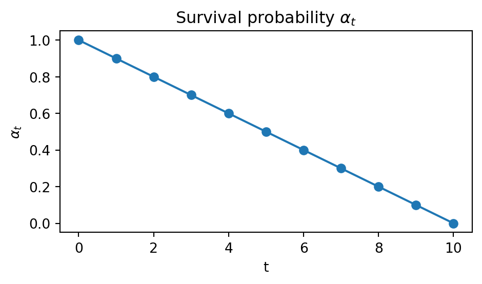

The code for backward sampling is basically the same, except for the number of if branch is now four, rather than just one.

def reverse_sample_pairs(num_samples: int, p_unmask: np.ndarray, T: int):
    x1 = np.full(num_samples, MASK, dtype=int)
    x2 = np.full(num_samples, MASK, dtype=int)
    hist1 = np.empty((T + 1, num_samples), dtype=int); hist1[0] = x1
    hist2 = np.empty((T + 1, num_samples), dtype=int); hist2[0] = x2

    for t in range(T, 0, -1):
        p = p_unmask[t-1]

        # both masked
        both = (x1 == MASK) & (x2 == MASK)
        idx = np.where(both)[0]
        if idx.size > 0:
            um1 = rng.random(idx.size) < p
            um2 = rng.random(idx.size) < p

            idx_both = idx[um1 & um2]
            if idx_both.size > 0:
                flat = pi_joint.ravel()
                choices = rng.choice(K*K, size=idx_both.size, p=flat)
                xs = choices // K; ys = choices % K
                x1[idx_both] = xs; x2[idx_both] = ys

            idx_only1 = idx[um1 & (~um2)]
            if idx_only1.size > 0:
                x1[idx_only1] = rng.choice(K, size=idx_only1.size, p=pi_x)

            idx_only2 = idx[(~um1) & um2]
            if idx_only2.size > 0:
                x2[idx_only2] = rng.choice(K, size=idx_only2.size, p=pi_y)

        # x1 masked, x2 revealed
        idx_b1 = np.where((x1 == MASK) & (x2 != MASK))[0]
        if idx_b1.size > 0:
            will = rng.random(idx_b1.size) < p
            idx_now = idx_b1[will]
            if idx_now.size > 0:
                y_vals = x2[idx_now]
                for val in np.unique(y_vals):
                    m = (y_vals == val); n = m.sum()
                    x1[idx_now[m]] = rng.choice(K, size=n, p=cond_x_given_y[val, :])

        # x2 masked, x1 revealed
        idx_b2 = np.where((x2 == MASK) & (x1 != MASK))[0]
        if idx_b2.size > 0:
            will = rng.random(idx_b2.size) < p
            idx_now = idx_b2[will]
            if idx_now.size > 0:
                x_vals = x1[idx_now]
                for val in np.unique(x_vals):
                    m = (x_vals == val); n = m.sum()
                    x2[idx_now[m]] = rng.choice(K, size=n, p=cond_y_given_x[val, :])

        hist1[T - t + 1] = x1; hist2[T - t + 1] = x2

    assert np.all(x1 != MASK) and np.all(x2 != MASK)
    return np.stack([x1, x2], axis=1), hist1, hist2

3.3 Honest Sampling

Again, using the exact backward kernel, we are able to reproduce the true joint distribution.

# Run
N = 100_000
pairs, h1, h2 = reverse_sample_pairs(N, p_unmask, T)

# Empirical joint
counts = np.zeros((K, K), dtype=float)
for a, b in pairs:
    counts[a, b] += 1.0
pi_emp = counts / counts.sum()

fig, ax = plt.subplots(1, 2, figsize=(8, 3.4))
im0 = ax[0].imshow(pi_joint, origin="lower", aspect="equal")
ax[0].set_title("True joint π_data")
ax[0].set_xlabel("x2"); ax[0].set_ylabel("x1")
for i in range(K):
    for j in range(K):
        ax[0].text(j, i, f'{pi_joint[i, j]:.3f}', 
                ha='center', va='center', color='white', fontsize=8)
fig.colorbar(im0, ax=ax[0], fraction=0.046, pad=0.04)

im1 = ax[1].imshow(pi_emp, origin="lower", aspect="equal")
ax[1].set_title("Empirical joint (reverse)")
ax[1].set_xlabel("x2"); ax[1].set_ylabel("x1")
for i in range(K):
    for j in range(K):
        ax[1].text(j, i, f'{pi_emp[i, j]:.3f}', 
                ha='center', va='center', color='white', fontsize=8)
fig.colorbar(im1, ax=ax[1], fraction=0.046, pad=0.04)

plt.tight_layout()
plt.show()

def l1_kl(pairs, split=10):
    chunks = np.array_split(pairs, split)
    l1, kl = [], []
    for chunk in chunks:
        counts = np.zeros((K, K), dtype=float)
        for a, b in chunk:
            counts[a, b] += 1.0
        pi_emp = counts / counts.sum()
        
        eps = 1e-12
        l1.append(np.abs(pi_emp - pi_joint).sum())
        nz = (pi_emp > 0) & (pi_joint > 0)
        kl.append((pi_emp[nz] * np.log((pi_emp[nz] + eps) / pi_joint[nz])).sum())
    return l1, kl

l1, kl = l1_kl(pairs)

print("L1 distance:", round(np.mean(l1), 6), " ± ", round(np.var(l1), 6), "   KL(emp || true):", f"{np.mean(kl):.6e} ± {np.var(kl):.6e}")

L1 distance: 0.024162  ±  4.6e-05    KL(emp || true): 7.286359e-04 ± 7.462192e-08

Note that since the survival rate \(\alpha_t\) decreases linearly, the number of newly unmasked coordinates per step will decrease exponentially.

new_unmasks_per_step = []
for t in range(T):
    changed1 = (h1[t] == MASK) & (h1[t+1] != MASK)
    changed2 = (h2[t] == MASK) & (h2[t+1] != MASK)
    new_unmasks_per_step.append(changed1.sum() + changed2.sum())

plt.figure(figsize=(6, 3))
plt.plot(range(1, T+1), new_unmasks_per_step, marker="o")
plt.title("Newly unmasked coordinates per step")
plt.xlabel("reverse step (t→t-1)")
plt.ylabel("#coords")
plt.tight_layout()
plt.show()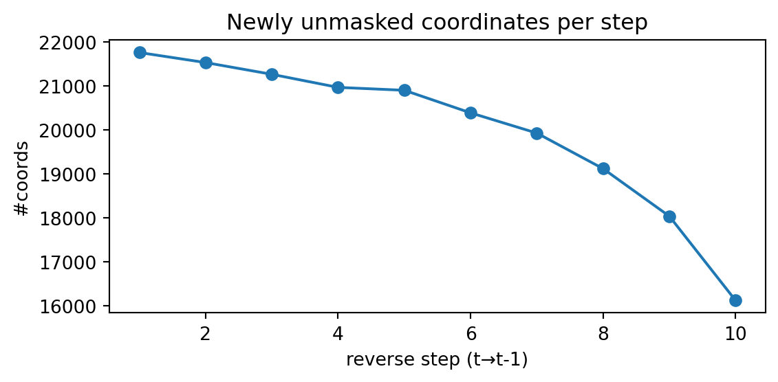

3.3.1 Larger Step Size

What if we employ a large step size?

Actually, the result doesn’t change. Moreover, the accuracy is higher, since it is equivalent to direct sampling from \(\pi_{\text{data}}\).

T = 1  # Number of steps
alpha = np.linspace(1.0, 0.0, T + 1)
p_unmask = (alpha[:-1] - alpha[1:]) / (1.0 - alpha[1:])
p_unmask = np.clip(p_unmask, 0.0, 1.0)

# Run
N = 100_000
pairs, h1, h2 = reverse_sample_pairs(N, p_unmask, T)

# Empirical joint
counts = np.zeros((K, K), dtype=float)
for a, b in pairs:
    counts[a, b] += 1.0
pi_emp = counts / counts.sum()

fig, ax = plt.subplots(1, 2, figsize=(8, 3.4))
im0 = ax[0].imshow(pi_joint, origin="lower", aspect="equal")
ax[0].set_title("True joint π_data")
ax[0].set_xlabel("x2"); ax[0].set_ylabel("x1")
for i in range(K):
    for j in range(K):
        ax[0].text(j, i, f'{pi_joint[i, j]:.3f}', 
                ha='center', va='center', color='white', fontsize=8)
fig.colorbar(im0, ax=ax[0], fraction=0.046, pad=0.04)

im1 = ax[1].imshow(pi_emp, origin="lower", aspect="equal")
ax[1].set_title("Empirical joint (reverse)")
ax[1].set_xlabel("x2"); ax[1].set_ylabel("x1")
for i in range(K):
    for j in range(K):
        ax[1].text(j, i, f'{pi_emp[i, j]:.3f}', 
                ha='center', va='center', color='white', fontsize=8)
fig.colorbar(im1, ax=ax[1], fraction=0.046, pad=0.04)

plt.tight_layout()
plt.show()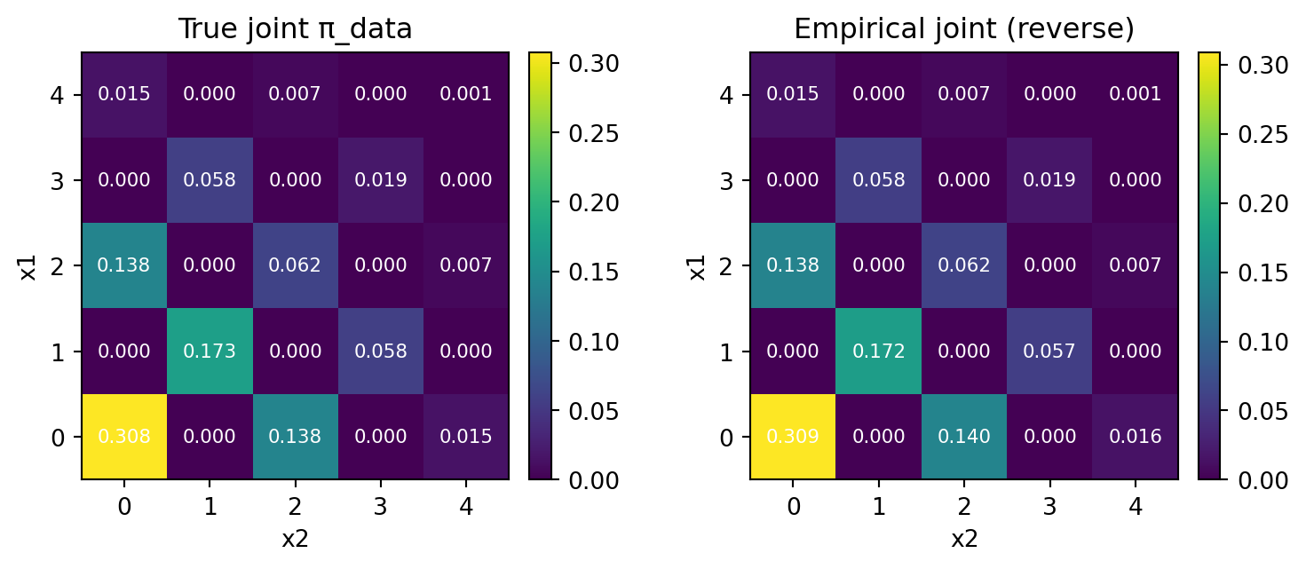

l1, kl = l1_kl(pairs)

print("L1 distance:", round(np.mean(l1), 6), " ± ", round(np.var(l1), 6), "   KL(emp || true):", f"{np.mean(kl):.6e} ± {np.var(kl):.6e}")

L1 distance: 0.021245  ±  5e-05    KL(emp || true): 6.510835e-04 ± 1.258177e-07

3.4 Coordinate-wise Sampling

The joint distribution would be unavailable, even if the learning based on the loss (1) were perfectly done, because of the product form assumption on the neural network predictor \(p_\theta\).³

We mock this situation by replacing the joint distribution in the exact kernel, programmed in Section 3.2, with the product of its marginals.

def reverse_sample_incorrect(num_samples: int, p_unmask: np.ndarray, T: int):
    x1 = np.full(num_samples, MASK, dtype=int)
    x2 = np.full(num_samples, MASK, dtype=int)
    hist1 = np.empty((T + 1, num_samples), dtype=int); hist1[0] = x1
    hist2 = np.empty((T + 1, num_samples), dtype=int); hist2[0] = x2

    for t in range(T, 0, -1):
        p = p_unmask[t-1]

        # both masked
        both = (x1 == MASK) & (x2 == MASK)
        idx = np.where(both)[0]
        if idx.size > 0:
            um1 = rng.random(idx.size) < p
            um2 = rng.random(idx.size) < p

            idx_both = idx[um1 & um2]
            if idx_both.size > 0:
                flat = np.outer(pi_x, pi_y).ravel()
                choices = rng.choice(K*K, size=idx_both.size, p=flat)
                xs = choices // K; ys = choices % K
                x1[idx_both] = xs; x2[idx_both] = ys

            idx_only1 = idx[um1 & (~um2)]
            if idx_only1.size > 0:
                x1[idx_only1] = rng.choice(K, size=idx_only1.size, p=pi_x)

            idx_only2 = idx[(~um1) & um2]
            if idx_only2.size > 0:
                x2[idx_only2] = rng.choice(K, size=idx_only2.size, p=pi_y)

        # x1 masked, x2 revealed
        idx_b1 = np.where((x1 == MASK) & (x2 != MASK))[0]
        if idx_b1.size > 0:
            will = rng.random(idx_b1.size) < p
            idx_now = idx_b1[will]
            if idx_now.size > 0:
                y_vals = x2[idx_now]
                for val in np.unique(y_vals):
                    m = (y_vals == val); n = m.sum()
                    x1[idx_now[m]] = rng.choice(K, size=n, p=cond_x_given_y[val, :])

        # x2 masked, x1 revealed
        idx_b2 = np.where((x2 == MASK) & (x1 != MASK))[0]
        if idx_b2.size > 0:
            will = rng.random(idx_b2.size) < p
            idx_now = idx_b2[will]
            if idx_now.size > 0:
                x_vals = x1[idx_now]
                for val in np.unique(x_vals):
                    m = (x_vals == val); n = m.sum()
                    x2[idx_now[m]] = rng.choice(K, size=n, p=cond_y_given_x[val, :])

        hist1[T - t + 1] = x1; hist2[T - t + 1] = x2

    assert np.all(x1 != MASK) and np.all(x2 != MASK)
    return np.stack([x1, x2], axis=1), hist1, hist2

T = 10  # Number of steps
alpha = np.linspace(1.0, 0.0, T + 1)
p_unmask = (alpha[:-1] - alpha[1:]) / (1.0 - alpha[1:])
p_unmask = np.clip(p_unmask, 0.0, 1.0)

pairs, h1, h2 = reverse_sample_incorrect(N, p_unmask, T)

# Empirical joint
counts = np.zeros((K, K), dtype=float)
for a, b in pairs:
    counts[a, b] += 1.0
pi_emp = counts / counts.sum()

fig, ax = plt.subplots(1, 2, figsize=(8, 3.4))
im0 = ax[0].imshow(pi_joint, origin="lower", aspect="equal")
ax[0].set_title("True joint π_data")
ax[0].set_xlabel("x2"); ax[0].set_ylabel("x1")
for i in range(K):
    for j in range(K):
        ax[0].text(j, i, f'{pi_joint[i, j]:.3f}', 
                ha='center', va='center', color='white', fontsize=8)
fig.colorbar(im0, ax=ax[0], fraction=0.046, pad=0.04)

im1 = ax[1].imshow(pi_emp, origin="lower", aspect="equal")
ax[1].set_title("Empirical joint (reverse)")
ax[1].set_xlabel("x2"); ax[1].set_ylabel("x1")
for i in range(K):
    for j in range(K):
        ax[1].text(j, i, f'{pi_emp[i, j]:.3f}', 
                ha='center', va='center', color='white', fontsize=8)
fig.colorbar(im1, ax=ax[1], fraction=0.046, pad=0.04)

plt.tight_layout()
plt.show()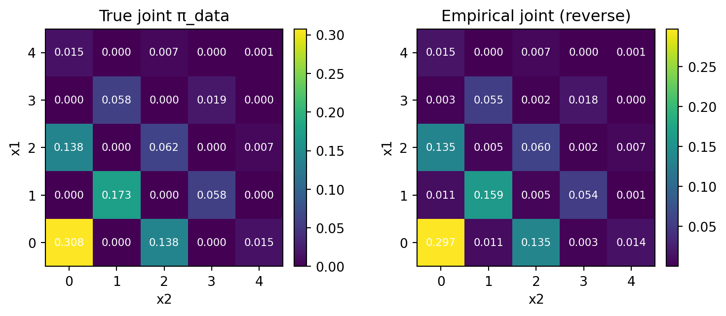

Then, this time the result is not so good.

l1, kl = l1_kl(pairs)

print("L1 distance:", round(np.mean(l1), 6), " ± ", round(np.var(l1), 6), "   KL(emp || true):", f"{np.mean(kl):.6e} ± {np.var(kl):.6e}")

L1 distance: 0.089135  ±  1.2e-05    KL(emp || true): -4.100716e-02 ± 6.515707e-06

There is a small deviation from the exact kernel, where \(\ell^1\) distance was \(0.024\pm0.00005\).

We can easily see, in the empirical distribution, some cells are assinged with positive mass, although the true probability is \(0\).

This effect becomes smaller when the number of steps T is large. For example, setting T=1000 gives us with almost same accuracy as the exact kernel (although we don’t show it here for brevity).

3.4.1 Larger Step Size

The situation gets worse when the step size is large, for example T=1.

T = 1  # Number of steps
alpha = np.linspace(1.0, 0.0, T + 1)
p_unmask = (alpha[:-1] - alpha[1:]) / (1.0 - alpha[1:])
p_unmask = np.clip(p_unmask, 0.0, 1.0)

pairs, h1, h2 = reverse_sample_incorrect(N, p_unmask, T)

# Empirical joint
counts = np.zeros((K, K), dtype=float)
for a, b in pairs:
    counts[a, b] += 1.0
pi_emp = counts / counts.sum()

fig, ax = plt.subplots(1, 2, figsize=(8, 3.4))
im0 = ax[0].imshow(pi_joint, origin="lower", aspect="equal")
ax[0].set_title("True joint π_data")
ax[0].set_xlabel("x2"); ax[0].set_ylabel("x1")
for i in range(K):
    for j in range(K):
        ax[0].text(j, i, f'{pi_joint[i, j]:.3f}', 
                ha='center', va='center', color='white', fontsize=8)
fig.colorbar(im0, ax=ax[0], fraction=0.046, pad=0.04)

im1 = ax[1].imshow(pi_emp, origin="lower", aspect="equal")
ax[1].set_title("Empirical joint (reverse)")
ax[1].set_xlabel("x2"); ax[1].set_ylabel("x1")
for i in range(K):
    for j in range(K):
        ax[1].text(j, i, f'{pi_emp[i, j]:.3f}', 
                ha='center', va='center', color='white', fontsize=8)
fig.colorbar(im1, ax=ax[1], fraction=0.046, pad=0.04)

plt.tight_layout()
plt.show()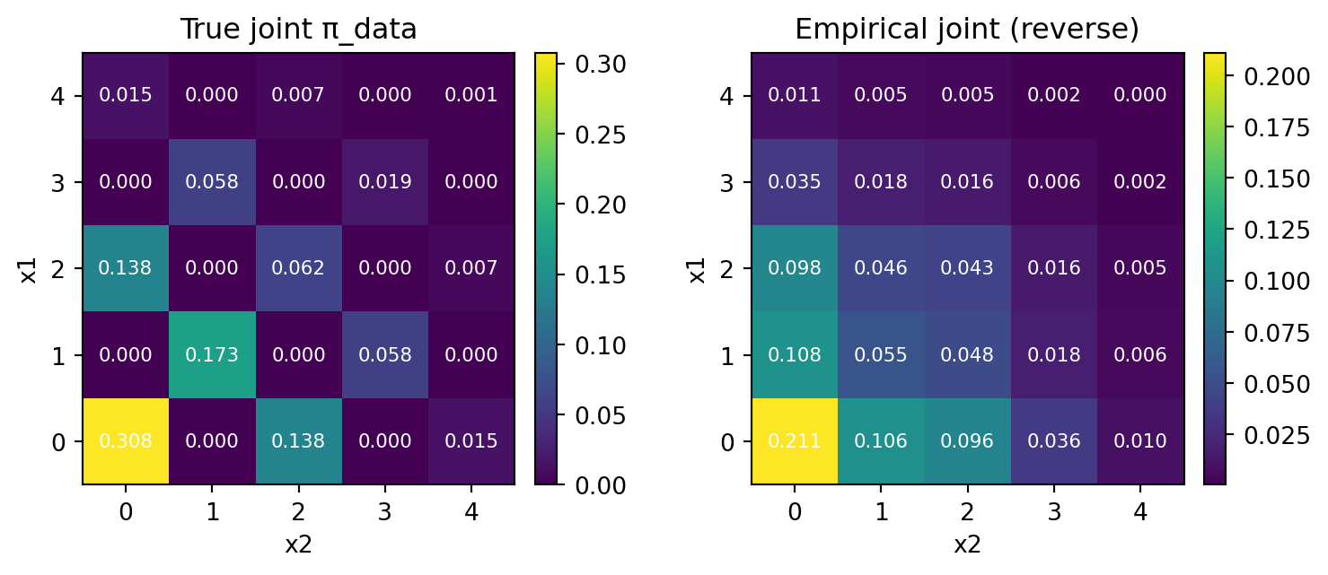

l1, kl = l1_kl(pairs)

print("L1 distance:", round(np.mean(l1), 6), " ± ", round(np.var(l1), 6), "   KL(emp || true):", f"{np.mean(kl):.6e} ± {np.var(kl):.6e}")

L1 distance: 0.85124  ±  4.4e-05    KL(emp || true): -2.884951e-01 ± 1.114368e-05

The error is now significant, because the incorrect product kernel is used every time, as we set \(T=1\) meaning unmasking in just one step!

One way to fix this is to set T as large as possible, making sure no more than one jump occurs simultaneously.

3.5 Corrector Sampling

Another remedy is to utilise Gibbs sampling ideas to correct the bias, again at the expense of computational cost.

To do this, we must identify a Markov kernel that keeps the marginal distribution of \(X_t\) invariant for every timestep \(t\in[0,1]\).

In our case, let us simply add a re-masking step, only to those pairs \((x_t^1,x_t^2)\)’s which are completely unmasked.

As there is some probability of having been unmasked simultaneously, re-masking only one of them, this time \(x_t^1\), will allow us a second chance to arrive at a correct pair \((x_t^{1,\text{corrected}},x_t^2)\).

def reverse_sample_corrector(num_samples: int, p_unmask: np.ndarray, T: int):
    x1 = np.full(num_samples, MASK, dtype=int)
    x2 = np.full(num_samples, MASK, dtype=int)
    hist1 = np.empty((T + 1, num_samples), dtype=int); hist1[0] = x1
    hist2 = np.empty((T + 1, num_samples), dtype=int); hist2[0] = x2

    for t in range(T, 0, -1):
        p = p_unmask[t-1]

        # both masked
        both = (x1 == MASK) & (x2 == MASK)
        idx = np.where(both)[0]
        if idx.size > 0:
            um1 = rng.random(idx.size) < p
            um2 = rng.random(idx.size) < p

            idx_both = idx[um1 & um2]
            if idx_both.size > 0:
                flat = np.outer(pi_x, pi_y).ravel()
                choices = rng.choice(K*K, size=idx_both.size, p=flat)
                xs = choices // K; ys = choices % K
                x1[idx_both] = xs; x2[idx_both] = ys

            idx_only1 = idx[um1 & (~um2)]
            if idx_only1.size > 0:
                x1[idx_only1] = rng.choice(K, size=idx_only1.size, p=pi_x)

            idx_only2 = idx[(~um1) & um2]
            if idx_only2.size > 0:
                x2[idx_only2] = rng.choice(K, size=idx_only2.size, p=pi_y)

        # x1 masked, x2 revealed
        idx_b1 = np.where((x1 == MASK) & (x2 != MASK))[0]
        if idx_b1.size > 0:
            will = rng.random(idx_b1.size) < p
            idx_now = idx_b1[will]
            if idx_now.size > 0:
                y_vals = x2[idx_now]
                for val in np.unique(y_vals):
                    m = (y_vals == val); n = m.sum()
                    x1[idx_now[m]] = rng.choice(K, size=n, p=cond_x_given_y[val, :])

        # x2 masked, x1 revealed
        idx_b2 = np.where((x2 == MASK) & (x1 != MASK))[0]
        if idx_b2.size > 0:
            will = rng.random(idx_b2.size) < p
            idx_now = idx_b2[will]
            if idx_now.size > 0:
                x_vals = x1[idx_now]
                for val in np.unique(x_vals):
                    m = (x_vals == val); n = m.sum()
                    x2[idx_now[m]] = rng.choice(K, size=n, p=cond_y_given_x[val, :])

        # corrector step
        q = 1.0 - p  # masking probability
        both = (x1 != MASK) & (x2 != MASK)
        idx = np.where(both)[0]
        if idx.size > 0:
            will = rng.random(idx.size) < q
            idx_now = idx[will]
            if idx_now.size > 0:
                x1[idx_now] = MASK
        # predictor step

        # both masked
        both = (x1 == MASK) & (x2 == MASK)
        idx = np.where(both)[0]
        if idx.size > 0:
            um1 = rng.random(idx.size) < p
            um2 = rng.random(idx.size) < p

            idx_both = idx[um1 & um2]
            if idx_both.size > 0:
                flat = np.outer(pi_x, pi_y).ravel()
                choices = rng.choice(K*K, size=idx_both.size, p=flat)
                xs = choices // K; ys = choices % K
                x1[idx_both] = xs; x2[idx_both] = ys

            idx_only1 = idx[um1 & (~um2)]
            if idx_only1.size > 0:
                x1[idx_only1] = rng.choice(K, size=idx_only1.size, p=pi_x)

            idx_only2 = idx[(~um1) & um2]
            if idx_only2.size > 0:
                x2[idx_only2] = rng.choice(K, size=idx_only2.size, p=pi_y)

        # x1 masked, x2 revealed
        idx_b1 = np.where((x1 == MASK) & (x2 != MASK))[0]
        if idx_b1.size > 0:
            will = rng.random(idx_b1.size) < p
            idx_now = idx_b1[will]
            if idx_now.size > 0:
                y_vals = x2[idx_now]
                for val in np.unique(y_vals):
                    m = (y_vals == val); n = m.sum()
                    x1[idx_now[m]] = rng.choice(K, size=n, p=cond_x_given_y[val, :])

        # x2 masked, x1 revealed
        idx_b2 = np.where((x2 == MASK) & (x1 != MASK))[0]
        if idx_b2.size > 0:
            will = rng.random(idx_b2.size) < p
            idx_now = idx_b2[will]
            if idx_now.size > 0:
                x_vals = x1[idx_now]
                for val in np.unique(x_vals):
                    m = (x_vals == val); n = m.sum()
                    x2[idx_now[m]] = rng.choice(K, size=n, p=cond_y_given_x[val, :])

        hist1[T - t + 1] = x1; hist2[T - t + 1] = x2

    assert np.all(x1 != MASK) and np.all(x2 != MASK)
    return np.stack([x1, x2], axis=1), hist1, hist2

T = 10  # Number of steps
alpha = np.linspace(1.0, 0.0, T + 1)
p_unmask = (alpha[:-1] - alpha[1:]) / (1.0 - alpha[1:])
p_unmask = np.clip(p_unmask, 0.0, 1.0)

pairs, h1, h2 = reverse_sample_corrector(N, p_unmask, T)

# Empirical joint
counts = np.zeros((K, K), dtype=float)
for a, b in pairs:
    counts[a, b] += 1.0
pi_emp = counts / counts.sum()

fig, ax = plt.subplots(1, 2, figsize=(8, 3.4))
im0 = ax[0].imshow(pi_joint, origin="lower", aspect="equal")
ax[0].set_title("True joint π_data")
ax[0].set_xlabel("x2"); ax[0].set_ylabel("x1")
for i in range(K):
    for j in range(K):
        ax[0].text(j, i, f'{pi_joint[i, j]:.3f}', 
                ha='center', va='center', color='white', fontsize=8)
fig.colorbar(im0, ax=ax[0], fraction=0.046, pad=0.04)

im1 = ax[1].imshow(pi_emp, origin="lower", aspect="equal")
ax[1].set_title("Empirical joint (reverse)")
ax[1].set_xlabel("x2"); ax[1].set_ylabel("x1")
for i in range(K):
    for j in range(K):
        ax[1].text(j, i, f'{pi_emp[i, j]:.3f}', 
                ha='center', va='center', color='white', fontsize=8)
fig.colorbar(im1, ax=ax[1], fraction=0.046, pad=0.04)

plt.tight_layout()
plt.show()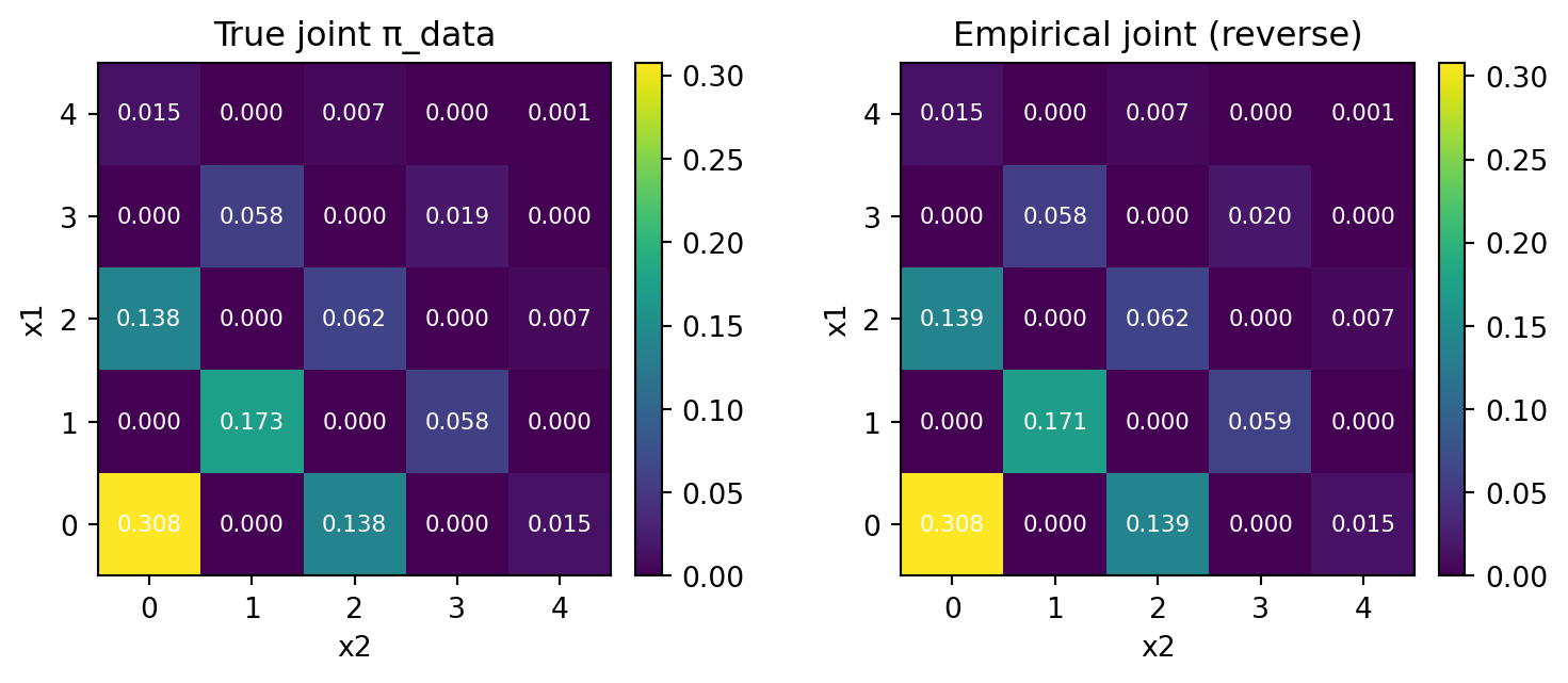

l1, kl = l1_kl(pairs, 10)

print("L1 distance:", round(np.mean(l1), 6), " ± ", round(np.var(l1), 6), "   KL(emp || true):", f"{np.mean(kl):.6e} ± {np.var(kl):.6e}")

L1 distance: 0.022518  ±  2e-05    KL(emp || true): 4.694469e-05 ± 8.500292e-08

We see a small improvement from the \(\ell^1\) distance of \(0.0241\). The difference is significant in terms of our variance of an order \(O(10^{-5})\) culculated from \(10\) repeated experiments.

This is the idea behind the predictor-corrector technique discussed, for example, in (Gat et al., 2024), (S. Zhao et al., 2024), (L. Zhao et al., 2024).

We only included one corrector step per reverse step, although more correction will increase accuracy.

This can be regarded as a form of inference time compute scaling (Wang et al., 2025), although it is a fairly bad idea to wait for the predictor-corrector steps to converge.

3.6 Discussion

Let us come back to the technique employed in (Chao et al., 2025), which we mentioned in Section 1.4.

As we have seen, the number of steps \(T\) has to be kept larger than \(d\), to make sure no more than one jump occurs simultaneously.

However, this increases the computational cost, as more time steps must be spent in simulating phantom jumps.

One thing we can do is to fill this blank steps with a informed ‘half-jump’, by introducing a sub-structure in each state \(x\in E\).

This half-jump is a bit more robust than a direct unmasking. Therefore we are able to spend the time up to \(T\) more meaningfully.

Thus, this strategy can be view as another way to mitigate the bias introduced by the incorrect backward kernel.

4 Future Works

Since the absorbing process is favoured only because of its time-agnostic property, its ability should be explained separately with the properties of the process.

4.1 A Reinforcenment Learning Take

The inference step and the sampling step should be decoupled, at least conceptually.

To tune the forward process noising schedule \(\alpha_t(x)\), a reinforcement learning framework will be employed, I believe in the near future.

This is a variant of meta-learning and, in this way, the unmasking network \(p_\theta\) will be able to efficiently learn the correct dependence structure in the data domain.

For example, in language modeling, there is a natural sequential structure, which is partly why autoregressive modeling has been dominant in this domain. However, by learning \(\alpha_t\) in masking process, a much more efficent factorization over texts can be aquired in a data-driven way.

I even think this \(\alpha_t\) can play an important role just as a word embedding does currently.

In the sampling step, a sampling time path planning will greatly enhance sample quality, just as Monte Carlo tree search does in reinforcement learning.

As a conclusion, the flexible framework of masked diffusion models will enable a marriage with reinforcement learning and meta learning, which will be a way to overcome the autoregressive modeling framework, because the latter imposes unnecessary sequential inductive bias into the model.

4.2 A Scaling Analysis

There are two papers, namely (Santos et al., 2023) and (Winkler et al., 2024), which carry out a scaling analysis as \(K\to\infty\), in order to bridge the gap between discrete and continuous state spaces.

In (Santos et al., 2023, sec. 2.4) and its Appendix C, it is proved that a fairly large class of discrete processes will converge to Ito processes, as \(K\to\infty\).

Their discussion based on a formal argument. They proves that the Kramers-Moyal expansion of the Chapman-Kolmogorov equation of the discrete process converges to that of a Ito process.

In other words, they didn’t identify the direct correspondence, for example deriving the exact expression of limiting SDEs.

(Winkler et al., 2024) builds on their analysis, identifying an OU process on \(\mathbb{R}^d\) corresponds to a Ehrenfest process.

This line of research has a lot to do with thermodynamics, and might provide insights into whether images should be modeled discretely or continuously.

Also, the limit \(d\to\infty\) has yet to be explored.

4.3 Concluding Remarks

I believe that masked diffusion modeling can be viewed as a form of Gibbs sampling, with a learned transition kernel.

Many current practices are based on (uniformly) random scan Gibbs, while the autoregressive models are a fixed scan Gibbs.

Most recent improvements are based upon ideas from reinforcement learning and meta learning, where an optimal order to unmask components is pursued.

This point of view might not be only an abstract nonsense. I actually believe that this point of view will be fruitful in the future.

5 関連記事

References

Arriola, M., Sahoo, S. S., Gokaslan, A., Yang, Z., Qi, Z., Han, J., … Kuleshov, V. (2025). Block diffusion: Interpolating between autoregressive and diffusion language models. In The thirteenth international conference on learning representations.

Campbell, A., Benton, J., De Bortoli, V., Rainforth, T., Deligiannidis, G., and Doucet, A. (2022). A Continuous Time Framework for Discrete Denoising Models. In S. Koyejo, S. Mohamed, A. Agarwal, D. Belgrave, K. Cho, and A. Oh, editors, Advances in neural information processing systems,Vol. 35, pages 28266–28279. Curran Associates, Inc.

Campbell, A., Yim, J., Barzilay, R., Rainforth, T., and Jaakkola, T. (2024). Generative Flows on Discrete State-Spaces: Enabling Multimodal Flows with Applications to Protein Co-Design.

Chao, C.-H., Sun, W.-F., Liang, H., Lee, C.-Y., and Krishnan, R. G. (2025). Beyond masked and unmasked: Discrete diffusion models via partial masking.

Gat, I., Remez, T., Shaul, N., Kreuk, F., Chen, R. T. Q., Synnaeve, G., … Lipman, Y. (2024). Discrete flow matching. In A. Globerson, L. Mackey, D. Belgrave, A. Fan, U. Paquet, J. Tomczak, and C. Zhang, editors, Advances in neural information processing systems,Vol. 37, pages 133345–133385. Curran Associates, Inc.

Kim, J., Shah, K., Kontonis, V., Kakade, S. M., and Chen, S. (2025). Train for the worst, plan for the best: Understanding token ordering in masked diffusions. In Forty-second international conference on machine learning.

Lezama, J., Salimans, T., Jiang, L., Chang, H., Ho, J., and Essa, I. (2023). Discrete predictor-corrector diffusion models for image synthesis. In The eleventh international conference on learning representations.

Liu, S., Nam, J., Campbell, A., Stark, H., Xu, Y., Jaakkola, T., and Gomez-Bombarelli, R. (2025). Think while you generate: Discrete diffusion with planned denoising. In The thirteenth international conference on learning representations.

Ou, J., Nie, S., Xue, K., Zhu, F., Sun, J., Li, Z., and Li, C. (2025). Your absorbing discrete diffusion secretly models the conditional distributions of clean data. In The thirteenth international conference on learning representations.

Peng, F. Z., Bezemek, Z., Patel, S., Rector-Brooks, J., Yao, S., Tong, A., and Chatterjee, P. (2025). Path planning for masked diffusion models with applications to biological sequence generation. In ICLR 2025 workshop on deep generative model in machine learning: Theory, principle and efficacy.

Rout, L., Caramanis, C., and Shakkottai, S. (2025). Anchored diffusion language model.

Santos, J. E., Fox, Z. R., Lubbers, N., and Lin, Y. T. (2023). Blackout diffusion: Generative diffusion models in discrete-state spaces. In A. Krause, E. Brunskill, K. Cho, B. Engelhardt, S. Sabato, and J. Scarlett, editors, Proceedings of the 40th international conference on machine learning,Vol. 202, pages 9034–9059. PMLR.

Shaul, N., Gat, I., Havasi, M., Severo, D., Sriram, A., Holderrieth, P., … Chen, R. T. Q. (2025). Flow matching with general discrete paths: A kinetic-optimal perspective. In The thirteenth international conference on learning representations.

Shi, J., Han, K., Wang, Z., Doucet, A., and Titsias, M. (2024). Simplified and generalized masked diffusion for discrete data. In A. Globerson, L. Mackey, D. Belgrave, A. Fan, U. Paquet, J. Tomczak, and C. Zhang, editors, Advances in neural information processing systems,Vol. 37, pages 103131–103167. Curran Associates, Inc.

Wang, G., Schiff, Y., Sahoo, S. S., and Kuleshov, V. (2025). Remasking discrete diffusion models with inference-time scaling. In ICLR 2025 workshop on deep generative model in machine learning: Theory, principle and efficacy.

Winkler, L., Richter, L., and Opper, M. (2024). Bridging discrete and continuous state spaces: Exploring the ehrenfest process in time-continuous diffusion models. In Forty-first international conference on machine learning.

Zhao, L., Ding, X., Yu, L., and Akoglu, L. (2024). Unified discrete diffusion for categorical data.

Zhao, S., Brekelmans, R., Makhzani, A., and Grosse, R. (2024). Probabilistic inference in language models via twisted sequential monte carlo. In.

Zheng, K., Chen, Y., Mao, H., Liu, M.-Y., Zhu, J., and Zhang, Q. (2025). Masked diffusion models are secretly time-agnostic masked models and exploit inaccurate categorical sampling. In The thirteenth international conference on learning representations.

Footnotes

1. Discrete Flow Matching (Campbell et al., 2024), (Gat et al., 2024), (Shaul et al., 2025) and simplified Masked diffusion (Shi et al., 2024), (Ou et al., 2025), (Zheng et al., 2025) are different frameworks with different ranges, but both lead to the same training objective (1), when applied to the forward masking process.

2. In the context of language modeling, the perplexity is defined as \(2^{l}\) where \(l\) is the average log-likelihood of the test set.

3. Of course, the exact sampling would have been available, for exmple, if we learned the backward intensity as (Campbell et al., 2022). However, these methods have been marginalized due to suboptimal performance.