階層モデル再論

多変量解析から機械学習へ

Statistics
Kernel
Probability
Bayesian
Author

司馬博文

Published

8/12/2024

Modified

8/14/2024

概要
本稿では,線型かつ1層の潜在変数モデルに議論を限り,機械学習と統計学と種々の応用分野での潜在変数モデル/階層モデルの議論を統一的に扱う.

はじめに

潜在変数模型とはどうやらとんでもなく広い射程を持った対象であるようである.

潜在変数モデルとは……
  1. 心理学,経済学をはじめとして多くの分野で中心的に扱われてきたモデルである(構造方程式モデル,因子分析,同時方程式モデル,Probabilistic Graphical Model など).
  2. ベイズ統計学では 階層モデル (hierarchical model) として極めて重要な役割を果たす.
  3. 生成モデリング(VAE, EBM, Diffusion, GAN)も,観測変数上の周辺分布がデータ分布に近づくように潜在変数模型を学習する方法である.
  4. 表現学習や独立成分分析だけでなく,脳も潜在変数模型に基いてメンタルモデルを構成しているという仮説もある(InfoMax に関する稿も参照).
  5. 情報理論において,通信路は潜在変数模型としてモデリングできる.この方向には,潜在変数模型は数学的には確率空間の圏上の図式であるとして研究されている (Perrone, 2024)

このように種々の文脈で登場する潜在変数模型であるが,それぞれの文脈において「潜在変数」の果たす役割は全く違う

しかし,数学的には全く同じ枠組みで記述できる.従って,そのように扱うことは一定の価値を持つだろう.

実際,近年になり,これから本稿で解説するように,潜在変数モデルの観点から心理学,経済学,環境科学,遺伝学,信号処理,逆問題,社会学,政治科学,マーケティング分野で独自に発展した手法が,特定の手法の特別な場合と見れるという理解が進み,手法の交流と知見の交換が進んでいる.

本稿の目的

本稿では主成分分析,因子分析,構造方程式モデリング,混合モデル,独立成分分析を,潜在変数モデルとして解釈し,図式で理解する

確率変数を丸つきの大文字で表し,\(X^i,Y^i\) は観測変数,\(Z^i\) は潜在変数を表す.矢印は 確率核 を表す.

混合モデル(第 4 節)

種々の 多変量解析法 を(ベイズ)階層モデルとして統一的に理解すると同時に,それぞれの文脈での「使い方の違い」に注目することを目指す.

1 主成分分析 (PCA)

1.1 はじめに

主成分分析では,\(p\) 次元のデータ \(\{x_i\}_{i=1}^n\subset\mathbb{R}^p\) の各成分を,より少数の潜在変数を持った1層の線型 Gauss 模型

で説明しようとする.1

歴史的に主成分分析は,おろした垂線の足の二乗距離和の意味でコストが最小になるような線型射影を求める問題 (Pearson, 1901) として最初に登場し,値の分散が最大となるような線型射影を求める問題 (Hotelling, 1933) として PCA の名前がつき,心理学分野,特に psychometrika で取り上げられて大きく発展した.

このような潜在変数モデルとしての見方は probabilistic PCA (Tipping and Bishop, 1999) / SPCA (Sensible PCA) (Roweis, 1997) として,因子分析から逆輸入する形で初めて自覚された見方である(第 2.3.1 節も参照).

確率的な見地から見れば,正規性を仮定した変数 \(Z^1,\cdots,Z^r\) の事前分布が互いに独立なデルタ分布に縮退している場合が古典的な PCA である (Roweis, 1997)

いずれの場合も追加の過程なくしてモデルは識別可能性がなく,後続タスクに応じて種々の制約を追加することで所望の解を得る,という動的な使い方がなされる.

以降,\(X\in\mathcal{L}(\Omega;\mathbb{R}^p),Z\in\mathcal{L}(\Omega;\mathbb{R}^r)\) を確率変数, \[ \boldsymbol{X}=(x_i^j)\in M_{n,p}(\mathbb{R}),\boldsymbol{Z}=(z_i^j)\in M_{n,r}(\mathbb{R}) \] を行列することに注意.

1.2 概要

PCA ではデータ行列を \[ \boldsymbol{X}:=\begin{pmatrix}x_1^\top\\\vdots\\x_n^\top\end{pmatrix}\in M_{n,p}(\mathbb{R}) \] で定めたとき,データ次元 \(p\) より小さい数の成分 \(r\) で説明しようとする: \[ \boldsymbol{X}\approx\boldsymbol{Z}C^\top,\qquad\boldsymbol{Z}:=\begin{pmatrix}z_1^\top\\\vdots\\z_n^\top\end{pmatrix}\in M_{n,r}(\mathbb{R}),C\in M_{p,r}(\mathbb{R}). \]

  • 古典的には,\(z_{ij}\) を(主成分)得点 (score),\(Z^i\)合成変量\(c_{ij}\)負荷量 (loading) ともいう (足立浩平 and 山本倫生, 2024)
  • 機械学習では \(Z^1,\cdots,Z^r\)潜在因子\(W\in M_{pr}(\mathbb{R})\)荷重 (weight) ともいう (Murphy, 2022)

この問題は \(\boldsymbol{X}\)特異値分解 (SVD) \(\boldsymbol{X}=U\Sigma V^\top\) により解ける: \[ \boldsymbol{Z}=U\Sigma_{1:r}^\alpha A=\boldsymbol{X}(\underbrace{V\Sigma^{\alpha-1}_{1:r}A}_{=:W}),\qquad C:=V\Sigma_{1:r}^{1-\alpha}(A^{-1})^\top. \] ただし,\(\alpha\in\mathbb{R},A\in\mathrm{GL}_p(\mathbb{R})\) は任意である.この解は,特異値分解の性質により,残差を Hilbert-Schmidt ノルムの意味で最小にする: \[ \min_C\|\boldsymbol{X}-\boldsymbol{Z}C^\top\|_\mathrm{HS}=\min_C\frac{1}{n}\sum_{i=1}^n\lvert x_i-Cz_i\rvert^2=\sigma_{r+1} \tag{1}\] この目的関数は復元誤差とも理解できる.ただし,\(\sigma_{r+1}\) は行列 \(\boldsymbol{Z}C\) の第 \(r+1\) 特異値である.

1.3 主成分分散最大化

荷重行列 \(W\)\(W^\top W=I_r\) を満たすという制約条件を追加すると,目的関数 (1) は潜在変数の分散を最大にすることと等価になる: \[ \operatorname*{argmin}_{W}\|\boldsymbol{X}-\boldsymbol{Z}W\|_\mathrm{HS}=\operatorname*{argmin}_W\operatorname{Tr}((\boldsymbol{X}W)^\top\boldsymbol{X}W). \tag{2}\]

すなわち,\(\boldsymbol{Z}=\boldsymbol{X}W\) の変動が差大になるようにすれば良い.

そのためには,確率変数 \(X\) のデータ行列 \(\boldsymbol{X}\) から計算した経験共分散行列 \(S\in M_{p}(\mathbb{R})_+\) の固有ベクトルのうち,対応する固有値が大きいものから \(w_1,\cdots,w_r\) として荷重行列とすれば良い: \[ W:=(w_1\;\cdots\;w_r). \]

実はこれは解の1つに過ぎず,\(W\) に右から直交行列を乗じて「回転」させたものは全て解になる.上の解は追加の条件 \(Z^\top Z=I_r\) を課すことで特定される.

1.4 計算上の注意

各次元に関する長さのスケールを揃えるために,PCA を始める前にデータを正規化しておくか,または共分散行列 \(S\) の代わりに,相関行列を用いるべきである.

また,実際に最適化や相関行列の固有値分解をすることはなく,基本的に SVD の方が \(O(np^2)+O(p^3)\) と高速である (Unkel and Trendafilov, 2010)

さらに次元 \(p\) が高い場合は,確率的 SVD (Halko et al., 2011), (Drineas and Mahoney, 2016) を用いてさらに \(O(nr^2)+(r^3)\) まで削減できる.このような手法は確率的数値解析と呼ばれる (Murray et al., 2023)

1.5 線型射影による次元縮約

\(W^\top W=I_r\) の仮定の下で,PCA の目的関数 (1) は,潜在変数の分散最大化 (2) と見れるのだった.

これは同じ仮定の下で,データ変数 \(X\) の最小誤差の線型射影を求める問題とも見れる: \[ \operatorname*{argmin}_W\|\boldsymbol{X}-\boldsymbol{Z}W\|_\mathrm{HS}=\operatorname*{argmin}_W\|\boldsymbol{X}-\boldsymbol{X}WW^\top\|_\mathrm{HS}. \]

なお,一般の行列 \(A\) について \(P_A=A(A^{-1}A)^+A^\top\)\(\mathrm{Im}\,A\) 上の直交射影になる.\(A\) が直交行列であるとき,\(P_A=AA^\top\) が成り立つ.

1.6 因子分析志向の主成分分析

因子分析では,\(Z^1,\cdots,Z^r\) を対等な因子と見て,それぞれのデータへの影響を調べたい.このような場合は, \[ \frac{1}{n}\boldsymbol{Z}^\top\boldsymbol{Z}=I_r \] が自然な制約になる.この際の解は,直交行列 \(T\in O_r(\mathbb{R})\) の違いを除いて, \[ \boldsymbol{Z}=\sqrt{n}UT,\qquad C=\frac{1}{\sqrt{n}}V\Sigma_{1:r}T,\qquad W=\sqrt{n}V\Sigma_{1:r}^{-1}T, \] まで確定する.

しばしば,追加の仮定 \[ C^\top C=\mathrm{diag}(\rho_{1:r}),\qquad \rho_1\ge\cdots\ge\rho_r\ge0 \] を課して得られる一意な解 \[ \boldsymbol{Z}=\sqrt{n}U,\qquad C=\frac{1}{\sqrt{n}}V\Sigma_{1:r},\qquad W=\sqrt{n}V\Sigma_{1:r}^{-1}, \]初期解 と呼び,これを「回転」させることで他の解が探索され,所望の分解を探す.

因子分析では (Thurstone, 1947) 以来,種々の回転法とアルゴリズムが蓄積している (足立浩平 and 山本倫生, 2024).一般にこの文脈では,(Thurstone, 1947) にいう「単純構造」を達成した,解釈が容易な因子をドメイン知識に基づいて構成することを目指す.この「単純構造」とは,現代でいう一種の disentangled factor と理解できる.

2 因子分析 (FA)

2.1 はじめに

主成分分析が「低階数近似」ならば,因子分析は「高階数近似」というべきである (足立浩平, 2023)

より正確には,因子分析は,観測の各次元 \(X^1,\cdots,X^p\) ごとに「独自因子」\(Z^1,\cdots,Z^p\) を想定しつつ,全観測に共通する「共通因子」\(F^1,\cdots,F^r\) をどのように抽出できるかを考える,という志向性を持つ:

この意味では,FA は独自因子 \(U^1,\cdots,U^p\) を追加した PCA とも理解できる.

歴史的には (Spearman, 1904) が古典テスト理論の文脈で \(r=1\) の因子分析を,(Thurstone, 1947) が一般の \(1\le r<p\) の場合の因子分析を「回転」の手法と共に導入した.

さらに興味深いことに,FA では PCA をはじめとした多くの多変量分析手法と違い,(Lawley, 1942), (Anderson and Rubin, 1956) らにより,初期から確率的な扱いが発展した手法である (足立浩平 and 山本倫生, 2024)

FA に倣う形で,PCA にも確率論的なアプローチが導入された (Tipping and Bishop, 1999), (Roweis, 1997)

2.2 概要

FA では \(\boldsymbol{Z}=(\boldsymbol{F}\;\boldsymbol{U})\in M_{n,r+p}(\mathbb{R})\) の分解に基づき, \[ \boldsymbol{X}\approx\boldsymbol{F}A^\top+\boldsymbol{U}\Psi^{1/2},\qquad A\in M_{r,p}(\mathbb{R}),\Psi=\mathrm{diag}(\psi_1,\cdots,\psi_p)\in M_p(\mathbb{R}), \] によってデータ行列 \(\boldsymbol{X}\in M_{n,p}(\mathbb{R})\) を説明しようとする.2

PCA よりさらに識別可能性は絶望的であるが,FA では潜在変数の解釈可能性担保のため,次の仮定を課す: \[ \boldsymbol{1}_n^\top\boldsymbol{F}=\boldsymbol{0}_r,\qquad \boldsymbol{1}_n^\top\boldsymbol{U}=\boldsymbol{0}_p, \] \[ \boldsymbol{F}^\top\boldsymbol{F}=n\boldsymbol{I}_r,\qquad \boldsymbol{U}^\top\boldsymbol{U}=n\boldsymbol{I}_p,\qquad\boldsymbol{F}^\top\boldsymbol{U}=O. \] すなわち,推定される確率変数 \(F,U\) が標準化されていて互いに無相関であるように誘導する.

また,\(\boldsymbol{U}\) の経験分散が \(\Psi\) になることに注意.

  • 古典的には,\(f_{ij}\) を共通因子,\(\psi_j\) を独自因子の 得点 (score),\(a_{ij}\)負荷量 (loading) ともいう (足立浩平 and 山本倫生, 2024)
  • 機械学習では \(Z^1,\cdots,Z^r\)潜在因子\(W\in M_{pr}(\mathbb{R})\)荷重 (weight) ともいう (Murphy, 2022)

この問題は,\(C:=(A\;\Psi^{1/2})\) と定めると,PCA と同じ問題 (1) に帰着される: \[ \min_C\|\boldsymbol{X}-\boldsymbol{Z}C^\top\|_\mathrm{HS}. \]

これはやはり特異値分解により解くことができる (De Leeuw, 2004)

解は直交行列による回転を除いても,やはり一意に定まらないようである.

2.3 確率的アプローチ

ここで, \[ U:=\begin{pmatrix}U^1\\\vdots\\U^p\end{pmatrix}\in\mathcal{L}(\Omega;\mathbb{R}^p),\qquad F:=\begin{pmatrix}F^1\\\vdots\\F^r\end{pmatrix}\in\mathcal{L}(\Omega;\mathbb{R}^r), \] を確率変数とすると, \[ X\approx AF+\Psi^{1/2}U \tag{3}\] によって \(X\) に確率モデルが誘導されることになる.

2.3.1 正規性の仮定

\(U,F\) に正規性の仮定をおけば,このモデルは EM アルゴリズムなどを用いて最尤推定できる (Rubin and Thayer, 1982), (Ghahramani and Hinton, 1996).このような最尤推定のアプローチは (Lawley, 1942) から考えられていた.

この見方が PCA にも応用された.追加の仮定 \[ A^\top A=I_{r},\qquad \Psi=\sigma^2I_p, \] の下での FA への確率論的アプローチを probabilistic PCA (Tipping and Bishop, 1999) / SPCA (Sensible PCA) (Roweis, 1997) という.

\(\sigma\to0\) の極限で古典的 PCA が回復される.

2.3.2 共分散構造分析

一方で,分布の仮定は課さず,\(X\) の経験分散 \(S\) を,式 (3) の右辺の共分散 \[ \Sigma:=AA^\top+\Psi \] となるべく近づけるように学習する方法もある.

例えば (Harman and Jones, 1966), (Harman and Fukuda, 1966) では,Hilbert-Schmidt ノルム \(\|S-\Sigma\|_\mathrm{HS}\) の最小化することで解を探索する方法が考慮された.

このように,データの共分散行列を低階数近似するアプローチは 共分散構造分析 (Bock and Bargmann, 1966) ともいう.

さらに,確率論的なアプローチは一般の構造方程式モデル (SEM, 次節 3 参照) へと発展 (Karl Gustav Jöreskog, 1970), (Sörbom, 1974), (Karl G. Jöreskog, 1978) し,現状,共分散構造分析は SEM の特別な場合と解される.3

2.4 スパース推定

FA のモデルは識別可能とは程遠く,解釈可能性が重要である.(Thurstone, 1947) は因子付加行列が「単純構造」を持つことを一つの指標としたが,現代的にはスパース推定の言葉で与えられた 完全単純構造 (Bernaards and Jennrich, 2003) を仮定することが増えてきた.

スパース PCA (Zou et al., 2006), (Ian T Jolliffe and Uddin, 2003) では,従来の SVD + 回転ではなく,LASSO 様の \(L^1\)-正則化項によって,解釈可能な因子付加行列を得ようとする.最終的に得られる目的関数は elastic net (Zou and Hastie, 2005) 様になる.

等価だが,自動関連度決定 (ARD) を用いた Bayesian PCA (Bishop, 1998), (Archambeau and Bach, 2008) や spike-and-slab (Rattray et al., 2009) など,スパース性を促す事前分布を用いることもできる.

2.5 その他の事前分布

非正規な事前分布(特に Laplace 分布やロジスティック分布などの裾の重いもの)を用いることで,モデルが識別可能性を回復することがある.

このように,一般の設定で潜在変数モデルが識別可能になるための条件が,非線型独立分析の分野で提案されている (Khemakhem et al., 2020)

2.5.1 Gamma 分布

また,Gamma 事前分布は非負かつスパースな表現を促進し,カウントデータとよく用いられる (Canny, 2004)

これは環境科学分野の Positive Matrix Factorization (Paatero and Tapper, 1994) や信号処理分野の Nonnegative Matrix Factorization (NMF) (Lee and Seung, 1999) の,確率論的な一般化と見れる (Buntine and Jakulin, 2006)

2.5.2 Dirichlet 分布

また,Dirichlet 事前分布を用いることで,潜在変数 \(Z\in\mathcal{L}(\Omega;\mathbb{R}^r)\)\[ \sum_{i=1}^rZ^i=1 \] が課されるため,「各次元への依存度」のような意味づけが可能になる.これは政治学における空間分析において,「どの立場への傾倒が強いか」を推定することにも用いられる (Buntine and Jakulin, 2006)

このモデルは multinomial PCA (Buntine and Jakulin, 2006) の他に,遺伝学で admixture (Pritchard et al., 2000),simplex factor analysis (Bhattacharya and Dunson, 2012), 科学出版で mixed-membership model (Erosheva et al., 2004),マーケティングで user rating profile model (Marlin, 2003) など,種々の分野で独立に提案されている.

2.6 非線型化

FA の一般化の方向性として,正規性の緩和の他に,線型性の緩和があり得る.

MCMC による推論 (Hoffman, 2017) をすることも,または指数型分布 (Collins et al., 2001) への拡張や,VAE による非線型化を通じて変分推論をすることも考えられる.

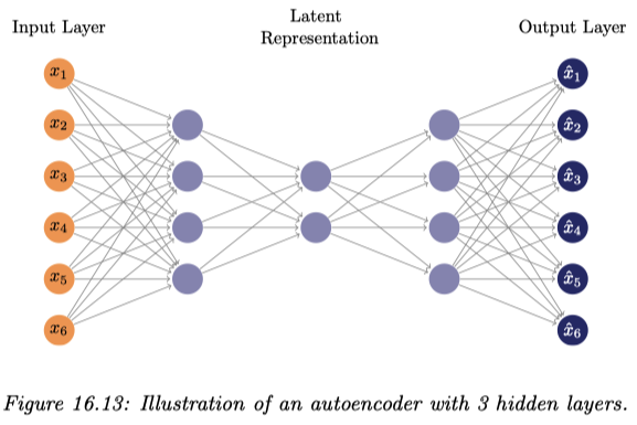
自己符号化器 は,まさに非線型な潜在変数モデルに対する最尤推定を行っており,4層以上のニューラルネットワークを用いることで PCA を非線型化して一般化することができる.4

また,カーネル法と Gauss 過程により非線型化することもできる (Lawrence, 2005)

2.7 混合モデリング

複数の線型 Gauss 因子分析モデルの重ね合わせとみなす mixture of factor analysers (Ghahramani and Hinton, 1996) も単純ながら表現が高く,EM アルゴリズムや SGD (Richardson and Weiss, 2018), (Zong et al., 2018) によって推定できる.

(Richardson and Weiss, 2018) では生成モデルとしての性能も GAN と劣らないこと,VAE や GAN などの生成モデルよりも分布へのフィッティングが良いことを報告している.

さらにこのアプローチはノンパラメトリックベイズ法につながる.この方法では,例えば (Paisley and Carin, 2009) では Beta 過程事前分布をおき,Gibbs サンプラーで推論することで,混合数 \(K\) も同時に自動で決定できる.

3 構造方程式モデリング (SEM)

3.1 はじめに

(K. G. Jöreskog, 1969) は因子分析モデルを潜在変数モデルとして,事前情報を取り入れるなど柔軟に用いた.

特に,データを(現代でいう)訓練データと検証データに分けて,因子分析により推定された潜在変数間の関数関係を検定するための方法を提案し (K. G. Jöreskog and Lawley, 1968),これを 検証的因子分析 (Confirmatory FA) と呼び,それ以前の手法に 探索的因子分析 というレトロニムを与えた.5

最終的に,潜在変数同士により一般的な関数関係も考慮したものなど多くの潜在変数モデルが,共分散構造に基づいた非線型数値最適化を推論エンジンとして統一的に推定できることに辿り着いた.6

このことに加えて,潜在変数間の関数関係に適切な仮定をおくことで,因果推論・高次の因子分析・分散分析など従来考慮されなかった新たなタスクにも適用可能であることも了解された (Karl G. Jöreskog, 1978), (Bentler, 1980)7

現代では特徴抽出,生成,表現学習にも用いられていると思うと感慨である.

これを 共分散構造分析 または 構造方程式モデリング (SEM: Structural Equation Modeling) という.8 心理学の文脈では,潜在変数のことを 構成概念 (construct) と呼び,潜在変数間は無関係とした従来の因果分析モデルを 測定方程式 と呼ぶ.9

3.2 部分最小自乗モデル (PLS)

PLS (Partial Least Square) モデル (K. G. Jöreskog and Wold, 1982), (Gustafsson, 2001) では,次のような潜在変数モデルを用いて,2つの構成概念間の因果関係を評価しようとする (豊田秀樹, 1991)

なお,パス図において,潜在変数から観測変数に矢印が伸びている場合,これは影響的指標と呼ばれ,観測のモデルと解され,誤差が入ることが想定される (豊田秀樹, 1991)10 逆の矢印は形成的指標という.

すなわち,PLS では,\(X^1,X^2,X^3,\cdots\) には,\(Z^1,Z^2,\cdots\) とは独立な独自因子が作用していると仮定されている.

このような仮定は,\(Y^1,Y^2,\cdots\) を被説明変数として,教師あり PCA (Yu et al., 2006) に有用である.

というのも,被説明変数のうち必ずしも \(Y^1,Y^2,\cdots\) に関係する要素が全てとは限らないために,\(Z^1,Z^2\) の間で間接的に回帰分析を行いたい場合に自然な設定である (Nounou et al., 2002)

3.3 構造方程式モデリングの発展

PLS において,潜在変数から構成概念への矢印が全て影響的であった場合,これは潜在因子の間に関係が仮定されていることを除いて,(探索的)因子分析と等価になる.

一般に,SEM は,潜在変数同士の関数関係も考慮した因子分析モデルだと理解できる.

このようなモデルは,社会学において 多重指標分析 と呼ばれていたモデルに相当し (白倉幸男, 1984) (清水和秋, 1989),経済学において 同時方程式モデル と呼ばれていたモデルに相当する (Bentler, 1980)11

加えて,心理学・行動計量学においても,多くの既存の多変量解析法(因子分析,パス解析,二段階抽出モデル,潜在構造分析,項目反応モデルな)はいずれも SEM の特殊な形だと解釈できることが自覚された (McArdle, 1984), (Muthén, 2002)

こうして SEM の名と LISREL プログラムの下で,多くの社会科学分野で使われていたモデルが,形式的にはほとんど等価であるという了解が形成されていった.

このことから,SEM は第二世代の多変量解析 (Fornell, 1985) とも評される.12

3.4 計算統計学という要素

構造方程式モデリングが普及した理由の一つとして,計算機統計学の発展とうまく合流した点が見逃せない.

そもそも Jöreskog は,因子分析を研究していた時期 (Karl G. Jöreskog, 1966) (K. G. Jöreskog, 1967) から,数値的な解法とコンピュータプログラムの開発にも重点を置いていた.特に,因子分析モデルを,DFP 法 に基づいて数値的に最尤推定する方法を提案した (K. G. Jöreskog, 1967)

SEM も,コンピュータプログラム LISREL (LInear Structural RELationships) (Jőreskog and Thiilo, 1972) の存在が,広い分野の人口に膾炙した要因として大きい (清水和秋, 1989), (Grimm and Yarnold, 2016)

構造方程式モデルがどのように因子分析,因果分析,共分散構造分析を統合し,LISREL プログラムと共に発展していたかは,(清水和秋, 1994) に大変わかりやすくまとまっている

3.5 正準相関分析 (CCA)

正準相関分析 (Hotelling, 1936) においては,2つの構成概念の間は相関関係で結び,すべての観測は形成的な影響を及ぼすとする(観測誤差は想定しない) (豊田秀樹, 1991)

このモデルでは \(X^1,X^2,X^3\) とその潜在要因 \(Z^1\)\(X^4,X^5\) とその潜在要因 \(Z^2\) とを完全に対等に扱い,その間の関係を理解しようとする.

例えばマルチモーダル学習において,\(X,Y\) が類似したタスクに関するデータという場合に応用がある (岩瀬智亮 and 中山英樹, 2016).また,PLS と共に特徴抽出にも用いられる (Sun et al., 2009)

複数の標本に対して同時に実行する主成分分析ともみなせるが,別々に PCA を実行した場合と違い「共通要因」を抽出することに志向がある (赤穂昭太郎, 2013)

なお,正準相関分析が,このような確率論的解釈ができることは (Bach and Jordan, 2005) で自覚されたことである.

この潜在変数モデルとしての観点から,\(Z^3,Z^4,\cdots\) がある GCCA (Generalized CCA) (Horst, 1961),指数分布族の場合 (Klami et al., 2010),ニューラルネットワークにより非線型にした DCCA (Andrew et al., 2013),さらに変分推論する場合 (Wang et al., 2017), (Suzuki et al., 2017) に拡張されている.

質的データをダミーベクトルに変換して(一般化)正準相関分析を行う,質的データの解析法を 対応分析 (correspondence analysis) または 数量化第III類 ともいう.13

4 混合モデル (MM)

4.1 はじめに

混合モデルは,次のようなたいへん基本的な設定であるが,第 2.7 節で見たように,例えば因子分析モデルと組み合わせることで極めて豊かな表現力を持つ.

混合モデルは SEM の別の選択肢としても使える.また,ランダム効果要因を明示的にモデルに組み込む意味で,一般線型モデルの確率論的な拡張と考えることもできる (狩野裕, 2002)14

4.2 正規混合モデル (GMM)

\(Z\in\mathcal{L}(\Omega;[K])\)\[ [K]=\{1,\cdots,K\} \] に値を取る離散確率変数で,確率核 \(Z\to X\)\[ p(x|z=k)\,dx=\mathrm{N}_p(\mu_k,\Sigma_k) \] と表せる場合,\(X\) に課される仮定を 正規混合モデル (GMM: Gaussian Mixture Model) という.

\(Z\sim\mathrm{U}([K]),\Sigma_k=I\) の場合,これは \(K\)-平均クラスタリングに等価 なモデルとなる.

これは SGD により訓練をすることで,生成のタスクにおいても GAN に匹敵する性能も持つ (Richardson and Weiss, 2018)

また,デノイジングや deblurring, inpainting, super-resolution などの画像逆問題は,巨大な GMM の潜在変数の推定として理解できる (Zoran and Weiss, 2011), (Papyan and Elad, 2016)

4.3 正規スケール混合モデル (GSM)

Gaussian scale mixture モデルとは, \[ p(x|z)\,dx=\mathrm{N}_p(0,\sigma_0^2z) \] で定まる階層モデルである.

このモデルは,\(Z\) の分布により,種々の(特に裾の重い)分布を表せる:

  1. \(Z\sim\mathrm{Ber}(\pi)\) のときを spike and slab 分布という: \[ p(x)\,dx=\pi\mathrm{N}(0,\sigma_0^2)+(1-\pi)\delta_0. \]
  2. \(Z\sim\mathrm{C}(1)_+\) のとき,馬蹄分布 (Carvalho et al., 2010) という.15

4.4 潜在 Dirichlet 配分 (LDA)

4.4.1 はじめに

文書の埋め込み・数値表現を得るために,単語 \(i\in[M]\) が文書 \(j\in[N]\) に現れた回数をカウントした行列 \(\boldsymbol{C}\in M_{MN}(\mathbb{N})\) を通じた主成分分析が用いることも考えられる.

これを 潜在意味索引 (LSI: Latent Semantic Indexing) (Deerwester et al., 1990) と呼ぶ.得られた低次元埋め込みを文書検索 (document retrieval) などに用いることもできる.

\(\boldsymbol{C}\) の列も単語とし,帯幅 \(h>0\) を決めて,\(h\) 文字以内に単語 \(i,j\in[M]\) が共起した回数を \(C_{ij}\) とすると,全く同様の手続きが,単語の埋め込みに応用できる.これを 潜在意味解析 (LSA: Latent Semantic Analysis) (Deerwester et al., 1990) と呼ぶ.

4.4.2 確率的潜在意味索引 (PLSI)

(Hofmann, 1999) による pLSI または aspect model は LSI を確率モデル,特に混合モデルとして解釈し直したものである.

単語数よりも少ない数の トピック \(Z\) というものがあり,これが単語を決めている,というモデルを想定した.

このモデルを通じて,トピック \(Z\) の分布(あるいは,現代的には \(\Theta\) の値)を「文書」の特徴量とする,というアイデアである.

4.4.3 Dirichlet 事前分布の追加

変数 \(\Theta\) に Dirichlet 事前分布を追加し,完全なベイズの見方を提示したのが Latent Dirichlet Allocation (Blei et al., 2003) である.

\(\Theta\) を文書,\(Z\) トピック,\(W\) をトピックごとの語彙デッキとする.

最終的に,トピック \(Z\) とその人の語彙 \(W\) が合わさって,単語 \(X\) が観測されるというモデルが考えられている.

4.4.4 確率的トピックモデル

自然言語処理において,単語分布のモデリングの潜在変数は トピック と呼ばれて,これを確率的にモデリングする手法は PTM (Probabilistic Topic Model) (Blei, 2012) と呼ばれている.

「トピック」は短い文章の中でも激しく移り変わることが知られている (Church and Gale, 1991)

そのため,LDA では,\(\Theta\) の事前分布と \(W\) の事前分布は, \[ \mathrm{Dirichlet}(\alpha\boldsymbol{1}),\qquad\alpha>0, \] という形で,極めて小さい \(\alpha>0\) を設定し,特定のトピックがどの文書に現れるかは極めてスパースになるようにモデリングをする.

4.4.5 推論

LDA の推論手法には変分推論 (Blei et al., 2003) や Gibbs サンプリング (T. L. Griffiths and Steyvers, 2004),そしてスペクトルに基づく方法 (Arora et al., 2013) がある.

トピック数の決定には,尤度を 焼なまし重点サンプリング で計算する方法 (Wallach et al., 2009) の他,ノンパラメトリックベイズ法も用いられる (Yee Whye Teh and Blei, 2006)

4.4.6 時系列化

単語の並びは明らかな方向性があり,対照的なモデリングはこの消息を取り逃がしていると考えられる.

そこで,トピックの移り変わりを捉えるモデルとして dynamic topic model (Blei and Lafferty, 2006) がある.これは Kalman 平滑化と変分推論を組み合わせている様である.

また単語の時系列構造を捉えるために,LDA に隠れ Markov モデルを組み合わせた LDA-HMM (T. Griffiths et al., 2004) が提案された.TopicRNN (Dieng et al., 2017) ではより長距離の相関を捉えるために,RNN と組み合わせている.

4.5 状態空間モデル (SSM)

4.5.1 概要

状態空間モデル (State Space Model) は,混合モデルの時系列化と捉えられる:

潜在変数 \(X_t\) が離散的である場合は特に 隠れ Markov モデル (HMM: Hidden Markov Model) (Baum and Petrie, 1966) と呼ばれる.

HMM に関しては早くから EM 様の推定手法 Baum-Welch アルゴリズム (Baum and Eagon, 1967), (Baum et al., 1970) が提案されているが,データサイズが大きい場合は SGD が用いられる.Blocked Gibbs サンプラー (Scott, 2002) や,潜在変数を消去して,周辺尤度に関してスペクトル法/テンソル分解 (Hsu et al., 2012), (Animashree Anandkumar et al., 2012), (Anima Anandkumar et al., 2015), (Obermeyer et al., 2019) を実行するなどの代替手法がある.

4.5.2 構造的状態系列モデル (S4)

S4 (Structured State Space Sequence) (Gu et al., 2022), (Gu et al., 2020), (Goel et al., 2022) とは,時系列を深層ニューラルネットワークの力でモデリングするために,線型 Gauss で単純な SMM を上下にスタックし深層にしたものである.各層は LSSL (Linear State Space Layer) と呼ばれる.

さらに長距離の依存性に耐えるために,S5 (Smith et al., 2023) や Mamba (Gu and Dao, 2024) が提案されている.後者では,選択的に記憶を忘却できるような「選択」機構 (S6: Selective SSM) を導入している.

5 独立成分分析 (ICA)

5.1 はじめに

(線型)独立成分分析で用いるモデルは,PCA や FA のそれと全く変わらず,線型変換 \(x_n=Az_n\) でデータを説明しようとする:

ただし,潜在変数 \(Z^1,\cdots,Z^r\) は互いに 独立 であるという「真の構造」が強く想定される場合に使われる.

加えて,モデルの 識別可能性 を重視する.このために,(独立)因子分析(第 2.5 節)で考えたように,正規分布より裾の重い事前分布を導入することで,モデルの識別可能性を確約する.16

この意味で,確率モデルとしては PCA / FA に等価であるが,典型的な ICA の文脈では \(Z^1,\cdots,Z^r\) は非正規確率変数であり,\(A\) を生成荷重や混合行列,\(A^{-1}\)認識荷重 (recognition weight) などという.

5.2 推定手法

最初に 音源分離 について適用された (Bell and Sejnowski, 1995) では,\(X\)\(Z\) の相互情報量の最大化が目指された.

最尤推定は EM アルゴリズムの他に近似 Newton 法で実行されることもあり,fast ICA (Hyvärinen and Oja, 2000) と呼ばれる.

また古典的には,探索的データ解析で考案された 射影追跡 (PP: Projection Pursuit) (Friedman and Tukey, 1974) みたく,学習される \(Z\) の分布が Gauss からなるべく遠いように学習することも考えられた.

disentangled な表現を学習したい場面では,\(Z\) の成分同士の相関が最小になるように学習される; \[ \operatorname{KL}\left(\operatorname{P}^Z,\bigotimes_{j=1}^r\operatorname{P}^{Z_j}\right). \]

最小情報コピュラに基づく方法も提案されている (Bedford et al., 2016), (Sei and Yano, 2024)

他にも表現学習や認知科学の文脈を踏襲して,InfoMax やスパース符号化などの原則がある.

5.3 非線型化

非線型独立成分分析は,表現学習の文脈でも研究されている

おわりに

現代の深層生成モデルは,いずれも非線型な潜在変数モデルであると理解できる.

その意味で,次の記事は全て,本稿の続きであり,本稿は現代の機械学習の壮大な序章としても理解できる.

非線形性の他に本稿で扱わなかったものは深層モデルである.

だがそもそも,現代のニューラルネットワークが深層化したのは,単純で可微分なモジュール性を保ちながら表現力を高めるためのトリックであり,確率論的には本稿で扱ったモデルと等価であるはずである.

ニューラルネットワークの他にも,計算のために深層化したモデルを考える場面は多い.例えばアニーリングを用いた SMC サンプラー は,グラフカルモデル \(Z\to X\) の潜在変数 \(Z\) の推定を,人工的に時系列構造を見出して状態空間モデル 4.5 にあてはめてサンプリングしやすくする方法と言える.

しかし,確率核は射をなすのだから,全てのモデルは本質的には一層であるとみなすこともできるのである.

この見方をとった方が計算効率が上がるという例もある.例えば (Chen et al., 2024) では,トランスフォーマーの注意機構をランダム Fourier 特徴写像で近似し,Monte Carlo 法によって元のモデルと等価な計算を安価に行っている

ベイズ機械学習位相的機械学習 をはじめとした,丁寧なモデルへの理解が,これからも手法への統一した視点からの理解と,応用分野を横断した相互理解を促進してくれるのではないかと,筆者は意気込んでいる.

扱ったモデル一覧

(Murphy, 2023, p. 920) より,本稿で扱ったモデルのいくつかを含んだ,数式による一覧表.すでに図式による解説を受けた後だと,より見やすいだろう.\(\operatorname{Cat}(c|\boldsymbol{\pi})\) は確率ベクトル \(\boldsymbol{\pi}\) が定める質量関数を表す.

付録

ここでは,歴史を感じる引用をいくつか紹介したい.

心理測定学 (psychometrics) における因子分析,計量経済学 (econometrics) における同時方程式モデル (simultaneous equation models), そして生物測定学 (biometrics) におけるパス解析 (path analysis) を,共分散構造分析の下に統一化することが可能となった契機は,潜在変数 (latent variables) の概念である (Bentler, 1980)(清水和秋, 1989)

そして,異分野横断の知見交流が進んだ契機の一つは,LISREL プログラムの存在であった.(清水和秋, 1994) では,ETS での安定した研究環境が LISREL の継続的な保守を可能にして最終的には WINDOWS 上でも安定して提供され,これを用いることを通じて異分野を巻き込みながら構造方程式モデリングが発展していった様子が詳細に解説されている.LISREL はバージョン VI まである.

紹介した文献からもわかるように,この分野は最近になってやっと日本では注目されてようになってきた。 このように日本へのこの方法論の導入が遅れた理由の一つはソフト流通の問題にあると筆者は考えている。青木 (1988) や土田 (1988) が述べているように, LISREL は大型計算機の場合, アメリカ産のコンビュータでしかサポートしてくれないとのことである。(清水和秋, 1989)

そして現代はというと,計算機統計学と機械学習が先行し(過ぎ)ていると思える.

もしその通りならば,種々の科学への応用とそれぞれ固有の課題への特殊化が,これからの未来を彩ってくれるのかもしれない.

References

Anandkumar, Anima, Ge, R., Hsu, D., Kakade, S. M., and Telgarsky, M. (2015). Tensor decompositions for learning latent variable models (a survey for ALT). In K. Chaudhuri, C. GENTILE, and S. Zilles, editors, Algorithmic learning theory, pages 19–38. Cham: Springer International Publishing.
Anandkumar, Animashree, Hsu, D., and Kakade, S. M. (2012). A method of moments for mixture models and hidden markov models. In S. Mannor, N. Srebro, and R. C. Williamson, editors, Proceedings of the 25th annual conference on learning theory,Vol. 23, pages 33.1–33.34. Edinburgh, Scotland: PMLR.
Anderson, T. W., and Rubin, H. (1956). Statistical inference in factor analysis. In Proceedings of the thrid berkeley symposium on mathematical statistics and probability,Vol. 5, pages 111–150.
Andrew, G., Arora, R., Bilmes, J., and Livescu, K. (2013). Deep canonical correlation analysis. In S. Dasgupta and D. McAllester, editors, Proceedings of the 30th international conference on machine learning,Vol. 28, pages 1247–1255. Atlanta, Georgia, USA: PMLR.
Archambeau, C., and Bach, F. (2008). Sparse probabilistic projections. In D. Koller, D. Schuurmans, Y. Bengio, and L. Bottou, editors, Advances in neural information processing systems,Vol. 21. Curran Associates, Inc.
Arora, S., Ge, R., Halpern, Y., Mimno, D., Moitra, A., Sontag, D., … Zhu, M. (2013). A practical algorithm for topic modeling with provable guarantees. In S. Dasgupta and D. McAllester, editors, Proceedings of the 30th international conference on machine learning,Vol. 28, pages 280–288. Atlanta, Georgia, USA: PMLR.
Asher, H. B. (1983). Causal modelling,Vol. 3. 和訳は心理学者広瀬弘忠による『因果分析法』(朝倉書店,1980); SAGE Publications, Inc.
Bach, F. R., and Jordan, M. I. (2005). A probabilistic interpretation of canonical correlation analysis. University of California, Berkeley. Retrieved from https://statistics.berkeley.edu/tech-reports/688
Baum, L. E., and Eagon, J. A. (1967). An inequality with applications to statistical estimation for probabilistic functions of markov processes and to a model for ecology. Bulletin of the American Mathematical Society, 73(3), 360–363.
Baum, L. E., and Petrie, T. (1966). Statistical inference for probabilistic functions of finite state markov chains. The Annals of Mathematical Statistics, 37(6), 1554–1563.
Baum, L. E., Petrie, T., Soules, G., and Weiss, N. (1970). A maximization technique occurring in the statistical analysis of probabilistic functions of markov chains. The Annals of Mathematical Statistics, 41(1), 164–171.
Bedford, T., Daneshkhah, A., and Wilson, K. J. (2016). Approximate uncertainty modeling in risk analysis with vine copulas. Risk Analysis, 36(4), 792–815.
Bell, A. J., and Sejnowski, T. J. (1995). An Information-Maximization Approach to Blind Separation and Blind Deconvolution. Neural Computation, 7(6), 1129–1159.
Bentler, P. M. (1980). Multivariate analysis with latent variables: Causal modeling. Annual Review of Psychology, 31(Volume 31, 1980), 419–456. Journal Article.
Bernaards, C. A., and Jennrich, R. I. (2003). Orthomax rotation and perfect simple structure. Psychometrika, 68(4), 585–588.
Bhattacharya, A., and Dunson, D. B. (2012). Simplex factor models for multivariate unordered categorical data. Journal of the American Statistical Association, 107(497), 362–377.
Bishop, C. (1998). Bayesian PCA. In M. Kearns, S. Solla, and D. Cohn, editors, Advances in neural information processing systems,Vol. 11. MIT Press.
Blei, D. M. (2012). Probabilistic topic models. Commun. ACM, 55(4), 77–84.
Blei, D. M., and Lafferty, J. D. (2006). Dynamic topic models. In Proceedings of the 23rd international conference on machine learning, pages 113–120. New York, NY, USA: Association for Computing Machinery.
Blei, D. M., Ng, A. Y., and Jordan, M. I. (2003). Latent Dirichlet Allocation. Journal of Machine Learning Research, 3, 993–1022.
Bock, R. D., and Bargmann, R. E. (1966). Analysis of covariance structures. Psychometrika, 31(4), 507–534.
Buntine, W., and Jakulin, A. (2006). Discrete component analysis. In C. Saunders, M. Grobelnik, S. Gunn, and J. Shawe-Taylor, editors, Subspace, latent structure and feature selection, pages 1–33. Berlin, Heidelberg: Springer Berlin Heidelberg.
Canny, J. (2004). GaP: A factor model for discrete data. In Proceedings of the 27th annual international ACM SIGIR conference on research and development in information retrieval, pages 122–129. New York, NY, USA: Association for Computing Machinery.
Carvalho, C. M., Polson, N. G., and Scott, J. G. (2010). The horseshoe estimator for sparse signals. Biometrika, 97(2), 465–480.
Chen, H., Liu, Z., Wang, X., Tian, Y., and Wang, Y. (2024). DiJiang: Efficient large language models through compact kernelization.
Church, K. W., and Gale, W. A. (1991). Probability scoring for spelling correction. Statistics and Computing, 1(2), 93–103.
Collins, M., Dasgupta, S., and Schapire, R. E. (2001). A generalization of principal components analysis to the exponential family. In T. Dietterich, S. Becker, and Z. Ghahramani, editors, Advances in neural information processing systems,Vol. 14. MIT Press.
De Leeuw, J. (2004). Least squares optimal scaling of partially observed linear systems. In Recent developments on structural equation models. Springer Dordrecht.
Deerwester, S., Dumais, S. T., Furnas, G. W., Landauer, T. K., and Harshman, R. (1990). Indexing by latent semantic analysis. Journal of the American Society for Information Science, 41(6), 391–407.
Dieng, A. B., Wang, C., Gao, J., and Paisley, J. (2017). TopicRNN: A recurrent neural network with long-range semantic dependency. In International conference on learning representations.
Drineas, P., and Mahoney, M. W. (2016). RandNLA: Randomized numerical linear algebra. Commun. ACM, 59(6), 80–90.
Erosheva, E., Fienberg, S., and Lafferty, J. (2004). Mixed-membership models of scientific publications. Proceedings of the National Academy of Sciences, 101(suppl_1), 5220–5227.
Fornell, C. (1985). A second generation of multivariate analysis: Classification of methods and implications for marketing research. Business, Stephen M. Ross School, University of Michigan. Retrieved from https://hdl.handle.net/2027.42/35621
Friedman, J. H., and Tukey, J. W. (1974). A projection pursuit algorithm for exploratory data analysis. IEEE Transactions on Computers, C-23(9), 881–890.
Ghahramani, Z., and Hinton, G. E. (1996). The EM algorithm for mixtures of factor analyzers. Department of Computer Science, University of Toronto. Retrieved from https://www.cs.toronto.edu/~hinton/absps/tr96-1.html
Ghojogh, B., Ghodsi, A., Karray, F., and Crowley, M. (2022). Factor analysis, probabilistic principal component analysis, variational inference, and variational autoencoder: Tutorial and survey.
Goel, K., Gu, A., Donahue, C., and Re, C. (2022). It’s raw! Audio generation with state-space models. In K. Chaudhuri, S. Jegelka, L. Song, C. Szepesvari, G. Niu, and S. Sabato, editors, Proceedings of the 39th international conference on machine learning,Vol. 162, pages 7616–7633. PMLR.
Griffiths, T. L., and Steyvers, M. (2004). Finding scientific topics. Proceedings of the National Academy of Sciences, 101(suppl_1), 5228–5235.
Griffiths, T., Steyvers, M., Blei, D., and Tenenbaum, J. (2004). Integrating topics and syntax. In L. Saul, Y. Weiss, and L. Bottou, editors, Advances in neural information processing systems,Vol. 17. MIT Press.
Grimm, L. G., and Yarnold, P. R. (2016). 研究論文を読み解くための多変量解析入門 応用篇. Reading and Understanding MORE Multivariate Statistics (2020) の翻訳書; 北大路書房.
Gu, A., and Dao, T. (2024). Mamba: Linear-time sequence modeling with selective state spaces.
Gu, A., Dao, T., Ermon, S., Rudra, A., and Ré, C. (2020). HiPPO: Recurrent memory with optimal polynomial projections. In H. Larochelle, M. Ranzato, R. Hadsell, M. F. Balcan, and H. Lin, editors, Advances in neural information processing systems,Vol. 33, pages 1474–1487. Curran Associates, Inc.
Gu, A., Goel, K., and Re, C. (2022). Efficiently modeling long sequences with structured state spaces. In International conference on learning representations.
Gustafsson, M. G. (2001). A probabilistic derivation of the partial least-squares algorithm. Journal of Chemical Information and Computer Sciences, 41(2), 288–294. doi: 10.1021/ci0003909.
Halko, N., Martinsson, P. G., and Tropp, J. A. (2011). Finding structure with randomness: Probabilistic algorithms for constructing approximate matrix decompositions. SIAM Review, 53(2), 217–288.
Harman, H. H., and Fukuda, Y. (1966). Resolution of the heywood case in the minres solution. Psychometrika, 31(4), 563–571.
Harman, H. H., and Jones, W. H. (1966). Factor analysis by minimizing residuals (minres). Psychometrika, 31(3), 351–368.
Hoffman, M. D. (2017). Learning deep latent Gaussian models with Markov chain Monte Carlo. In D. Precup and Y. W. Teh, editors, Proceedings of the 34th international conference on machine learning,Vol. 70, pages 1510–1519. PMLR.
Hofmann, T. (1999). Probabilistic latent semantic indexing. In Proceedings of the 22nd annual international ACM SIGIR conference on research and development in information retrieval, pages 50–57. New York, NY, USA: Association for Computing Machinery.
Horst, P. (1961). Generalized canonical correlations and their applications to experimental data. Journal of Clinical Psychology, 17(4), 331–347.
Hotelling, H. (1933). Analysis of a complex of statistical variables into principal components. Journal of Educational Psychology, 24(6), 417–441.
Hotelling, H. (1936). Relations between two sets of variates. Biometrika, 27(3/4), 321–377.
Hsu, D., Kakade, S. M., and Zhang, T. (2012). A spectral algorithm for learning hidden markov models. Journal of Computer and System Sciences, 78(5), 1460–1480.
Hyvärinen, A., and Oja, E. (2000). Independent component analysis: Algorithms and applications. Neural Networks, 13(4), 411–430.
Ian T Jolliffe, N. T. T., and Uddin, M. (2003). A modified principal component technique based on the LASSO. Journal of Computational and Graphical Statistics, 12(3), 531–547.
Jöreskog, Karl G. (1966). UMLFA: A computer program for unrestricted maximum likelihood factor analysis. ETS. Retrieved from https://www.ets.org/research/policy_research_reports/publications/report/1966/iazh.html
Jöreskog, K. G. (1967). Some contributions to maximum likelihood factor analysis. Psychometrika, 32(4), 443–482.
Jöreskog, K. G. (1969). A general approach to confirmatory maximum likelihood factor analysis. Psychometrika, 34(2), 183–202.
Jöreskog, Karl Gustav. (1970). A general method for analysis of covariance structures. Biometrika, 57(2), 239–251.
Jöreskog, Karl G. (1978). Structural analysis of covariance and correlation matrices. Psychometrika, 43(4), 443–477.
Jöreskog, K. G., and Lawley, D. N. (1968). New methods in maximum likelihood factor analysis. British Journal of Mathematical and Statistical Psychology, 21(1), 85–96.
Jöreskog, K. G., and Wold, H. (1982). Systems under indirect observation: Causality, structure, prediction. In, pages 263–270. North-Holland.
Jőreskog, K. G., and Thiilo, M. van. (1972). LISREL: A General Computer Program for Estimating a Linear Structural Equation System Involving Multiple Indicators of Unmeasured Variables. ETS Research Bulletin Series, 1972(2), i–71.
Khemakhem, I., Kingma, D., Monti, R., and Hyvarinen, A. (2020). Variational autoencoders and nonlinear ICA: A unifying framework. In S. Chiappa and R. Calandra, editors, Proceedings of the twenty third international conference on artificial intelligence and statistics,Vol. 108, pages 2207–2217. PMLR.
Klami, A., Virtanen, S., and Kaski, S. (2010). Bayesian exponential family projections for coupled data sources. In Proceedings of the twenty-sixth conference on uncertainty in artificial intelligence, pages 286–293. Arlington, Virginia, USA: AUAI Press.
Lawley, D. N. (1942). XIV.—further investigations in factor estimation. Proceedings of the Royal Society of Edinburgh. Section A. Mathematical and Physical Sciences, 61(2), 176–185.
Lawrence, N. (2005). Probabilistic non-linear principal component analysis with gaussian process latent variable models. Journal of Machine Learning Research, 6(60), 1783–1816.
Lee, D. D., and Seung, H. S. (1999). Learning the parts of objects by non-negative matrix factorization. Nature, 401(6755), 788–791.
Marlin, B. M. (2003). Modeling user rating profiles for collaborative filtering. In S. Thrun, L. Saul, and B. Schölkopf, editors, Advances in neural information processing systems,Vol. 16. MIT Press.
McArdle, J. J. (1984). On the madness in his method: R. B. Cattell’s contributions to structural equation modeling. Multivariate Behavioral Research, 19(2-3), 245–267.
Murphy, K. P. (2022). Probabilistic machine learning: An introduction. MIT Press.
Murphy, K. P. (2023). Probabilistic machine learning: Advanced topics. MIT Press.
Murray, R., Demmel, J., Mahoney, M. W., Erichson, N. B., Melnichenko, M., Malik, O. A., … Dongarra, J. (2023). Randomized numerical linear algebra: A perspective on the field with an eye to software (No. UCB/EECS-2023-19). Retrieved from http://www2.eecs.berkeley.edu/Pubs/TechRpts/2023/EECS-2023-19.html
Muthén, B. O. (2002). Beyond SEM: General Latent Variable Modeling. Behaviormetrika, 29(1), 81–117.
Nounou, M. N., Bakshi, B. R., Goel, P. K., and Shen, X. (2002). Process modeling by bayesian latent variable regression. AIChE Journal, 48(8), 1775–1793.
Obermeyer, F., Bingham, E., Jankowiak, M., Pradhan, N., Chiu, J., Rush, A., and Goodman, N. (2019). Tensor variable elimination for plated factor graphs. In K. Chaudhuri and R. Salakhutdinov, editors, Proceedings of the 36th international conference on machine learning,Vol. 97, pages 4871–4880. PMLR.
Paatero, P., and Tapper, U. (1994). Positive matrix factorization: A non-negative factor model with optimal utilization of error estimates of data values. Environmetrics, 5(2), 111–126.
Paisley, J., and Carin, L. (2009). Nonparametric factor analysis with beta process priors. In Proceedings of the 26th annual international conference on machine learning, pages 777–784. New York, NY, USA: Association for Computing Machinery.
Papyan, V., and Elad, M. (2016). Multi-scale patch-based image restoration. IEEE Transactions on Image Processing, 25(1), 249–261.
Pearson, K. (1901). On lines and planes of closest fit to systems of points in space. Philosophical Magazine, 2(11), 559–572.
Perrone, P. (2024). Markov Categories and Entropy. IEEE Transactions on Information Theory, 70(3), 1671–1692.
Pritchard, J. K., Stephens, M., and Donnelly, P. (2000). Inference of Population Structure Using Multilocus Genotype Data. Genetics, 155(2), 945–959.
Rattray, M., Stegle, O., Sharp, K., and Winn, J. (2009). Inference algorithms and learning theory for bayesian sparse factor analysis. Journal of Physics: Conference Series, 197(1), 012002.
Richardson, E., and Weiss, Y. (2018). On GANs and GMMs. In S. Bengio, H. Wallach, H. Larochelle, K. Grauman, N. Cesa-Bianchi, and R. Garnett, editors, Advances in neural information processing systems,Vol. 31. Curran Associates, Inc.
Roweis, S. (1997). EM algorithms for PCA and SPCA. In M. Jordan, M. Kearns, and S. Solla, editors, Advances in neural information processing systems,Vol. 10. MIT Press.
Rubin, D. B., and Thayer, D. T. (1982). EM algorithms for ML factor analysis. Psychometrika, 47(1), 69–76.
Scott, S. L. (2002). Bayesian methods for hidden markov models. Journal of the American Statistical Association, 97(457), 337–351.
Sei, T., and Yano, K. (2024). Minimum information dependence modeling. Bernoulli, 30(4), 2623–2643.
Simon, H. (1957). Models of man; social and rational. Wiley.
Smith, J. T. H., Warrington, A., and Linderman, S. (2023). Simplified state space layers for sequence modeling. In The eleventh international conference on learning representations.
Socan, G. (2003). The incremental value of rank factor analysis (PhD thesis). Rijksuniversiteit Groningen.
Sörbom, D. (1974). A General Method for Studying Differences in Factor Means and Factor Structure between Groups. British Journal of Mathematical and Statistical Psychology, 27(2), 229–239.
Spearman, C. (1904). ’General intelligence,’ objectively determined and measured. The American Journal of Psychology, 15(2), 201–293.
Sun, L., Ji, S., Yu, S., and Ye, J. (2009). On the equivalence between canonical correlation analysis and orthonormalized partial least squares. In Proceedings of the 21st international joint conference on artificial intelligence, pages 1230–1235. San Francisco, CA, USA: Morgan Kaufmann Publishers Inc.
Suzuki, M., Nakayama, K., and Matsuo, Y. (2017). Joint multimodal learning with deep generative models.
Thurstone, L. L. (1947). Multiple factor analysis. University of Chicago Press.
Tipping, M. E., and Bishop, C. M. (1999). Probabilistic principle component analysis. Journal of the Royal Statistical Society. Series B (Statistical Methodology), 61(3), 611–622.
Unkel, S., and Trendafilov, N. T. (2010). Simultaneous parameter estimation in exploratory factor analysis: An expository review. International Statistical Review, 78(3), 363–382.
Wallach, H. M., Murray, I., Salakhutdinov, R., and Mimno, D. (2009). Evaluation methods for topic models. In Proceedings of the 26th annual international conference on machine learning, pages 1105–1112. New York, NY, USA: Association for Computing Machinery.
Wang, W., Yan, X., Lee, H., and Livescu, K. (2017). Deep variational canonical correlation analysis.
Wright, S. (1918). On the nature of size factors. Genetics, 3(4), 367.
Wright, S. (1921). Correlation and causation. Journal of Agricultural Reserach, 20, 557–585.
Yee Whye Teh, M. J. B., Michael I Jordan, and Blei, D. M. (2006). Hierarchical dirichlet processes. Journal of the American Statistical Association, 101(476), 1566–1581.
Yu, S., Yu, K., Tresp, V., Kriegel, H.-P., and Wu, M. (2006). Supervised probabilistic principal component analysis. In Proceedings of the 12th ACM SIGKDD international conference on knowledge discovery and data mining, pages 464–473. New York, NY, USA: Association for Computing Machinery.
Zong, B., Song, Q., Min, M. R., Cheng, W., Lumezanu, C., Cho, D., and Chen, H. (2018). Deep autoencoding gaussian mixture model for unsupervised anomaly detection. In International conference on learning representations.
Zoran, D., and Weiss, Y. (2011). From learning models of natural image patches to whole image restoration. In 2011 international conference on computer vision, pages 479–486.
Zou, H., and Hastie, T. (2005). Regularization and Variable Selection Via the Elastic Net. Journal of the Royal Statistical Society Series B: Statistical Methodology, 67(2), 301–320.
Zou, H., Hastie, T., and Tibshirani, R. (2006). Sparse principal component analysis. Journal of Computational and Graphical Statistics, 15(2), 265–286.
岩瀬智亮, and 中山英樹. (2016). 深層一般化正準相関分析. 情報処理学会第78回全国大会講演論文集, 2016(1), 183–184.
星野崇宏, 岡田謙介, and 前田忠彦. (2005). 構造方程式モデリングにおける適合度指標とモデル改善について : 展望とシミュレーション研究による新たな知見. 行動計量学, 32(2), 209–235.
江口真透. (1999). 概パラメトリック推測 - 柔らかなモデルの構築 -. 統計数理, 47(1), 29–48.
清水和秋. (1989). 検証的因子分析,LISRELそしてRAMの概要. 関西大学社会学部紀要, 20(2), 61–86.
清水和秋. (1994). JöreskogとSörbomによるコンピュータ・プログラムと構造方程式モデル. 関西大学社会学部紀要, 25(3), 1–41.
狩野裕. (2002). 構造方程式モデリングは,因子分析,分散分析,パス解析の すべてにとって代わるのか?. 行動計量学, 29(2), 138–159.
甘利俊一,狩野裕,佐藤俊哉,松山裕,竹内啓,石黒真木夫. (2002). 多変量解析の展開:隠れた構造と因果を推理する,Vol. 5. 岩波書店.
白倉幸男. (1984). 多重指標線形構造モデルとその応用 : 研究ノート. 大阪大学人間科学部紀要, 10, 25–45.
豊田秀樹. (1991). 共分散構造分析の下位モデルとその適用例. 教育心理学研究, 39(4), 467–478.
豊田秀樹. (1992). SASによる共分散構造分析,Vol. 3. 東京大学出版会.
豊田秀樹. (2007). 共分散構造分析[理論編]. 朝倉書店.
赤穂昭太郎. (2013). 正準相関分析入門. 日本神経回路学会誌, 20(2), 62–72.
足立浩平. (2023). 50歳を超えてから始めた因子分析. 日本行動計量学会報, 177.
足立浩平, 伊藤真道, and 宇野光平. (2019). 行列分解に基づく因子分析とその新展開. 計算機統計学, 32(1), 61–77.
足立浩平, and 山本倫生. (2024). 主成分分析と因子分析―特異値分解を出発点として―. 共立出版.

Footnotes

  1. 図を見やすくするために,\(X^1\to X^{p-1}\)\(X^2\to X^p\) などは省略している.↩︎

  2. (足立浩平 and 山本倫生, 2024), (足立浩平, 2023) によると,この行列分解による定式化は Henk A. K. Kiers によるもので,初出は同大学からの博士論文 (Socan, 2003) が最初ではないか,とのこと.この見方を MDFA (Matrix Decomposition Factor Analysis) と呼ぶ.(足立浩平 et al., 2019) も参照.↩︎

  3. ただし,(星野崇宏 et al., 2005) は SEM をより一般的とし,共分散構造分析とは観測変数が連続な場合の下位モデルである,と解している.↩︎

  4. (江口真透, 1999) 第3節に,PCA をニューラルネットワークにより近似的に実行する方法が紹介されている.(Ghojogh et al., 2022) はサーベイを与えている.↩︎

  5. (豊田秀樹, 1992) では CFA を確認的因子分析と呼んでいる.(豊田秀樹, 1991) では,古典テスト理論を確認的因子分析の下位モデルとして紹介している.また,このような因果関係の確認的方法は,社会学における (Simon, 1957) の基準などが知られていた.↩︎

  6. (Karl Gustav Jöreskog, 1970) は具体的なモデルを例に取り,彼の検証的因果分析が,パス解析 (Wright, 1918), (Wright, 1921) のように因果分析に応用できることを示した結果だと言える (Asher, 1983).この観点から,パス解析は「検証的因果推論」と表現することもできる (甘利俊一,狩野裕,佐藤俊哉,松山裕,竹内啓,石黒真木夫, 2002, p. 73)↩︎

  7. (狩野裕, 2002) は SEM の射程と得意・不得意を分析している.↩︎

  8. 現代ではコンピュータの力により,新たに「生成」「表現学習」というタスクが加わったと思うと,感慨深い.↩︎

  9. (清水和秋, 1989), (豊田秀樹, 1992), (甘利俊一,狩野裕,佐藤俊哉,松山裕,竹内啓,石黒真木夫, 2002, p. 82) も参照.↩︎

  10. また,パス図では観測変数は四角で囲むべきであるが,ここでは省略した.↩︎

  11. 同時方程式は潜在変数を持たない模型で,経済学におけるパス解析の継承と見れる (豊田秀樹, 2007).特に Keynes 経済学におけるマクロな経済計画の発想で,Cowles 委員会 により 1940 年代から 1950 年代にかけて盛んに研究された.↩︎

  12. 多変量解析の高級言語とか形容することもあるという.構造方程式モデリングについては,(豊田秀樹, 1991), (狩野裕, 2002) も参照.↩︎

  13. オランダ学派を中心に等質性分析とも呼ぶ.↩︎

  14. ただし,SEM は共分散構造,混合モデルは平均構造に分析の焦点がある,という志向の違いもある.(狩野裕, 2002) も参照.↩︎

  15. \(\mathrm{C}(\sigma)_+\) は Cauchy 分布 \(\mathrm{C}(0,\sigma)\)\(\mathbb{R}_+\) 上に制限したものである.truncated Cauchy または half-Cauchy という.↩︎

  16. (Hyvärinen and Oja, 2000) では,(Bell and Sejnowski, 1995) のように測定誤差を考えない場合を ICA といい,誤差も入る一般の場合を IFA (Independent Factor Analysis) と呼び分けている.(甘利俊一,狩野裕,佐藤俊哉,松山裕,竹内啓,石黒真木夫, 2002, p. 110) も参照.「これを回転の不定性という.因子分析はさまざまな考察によって,この不定性を解消しようとする.独立成分分析は,非正規性を仮定すれば,この不定性が消えることを示したものとも言える」(甘利俊一,狩野裕,佐藤俊哉,松山裕,竹内啓,石黒真木夫, 2002, p. 13)↩︎