カーネル法の概観

関連ページ

A Blog Entry on Bayesian Computation by an Applied Mathematician

$$

$$

1 半正定値カーネル

1.1 はじめに

カーネル法は，カーネルの選択と構成が第一歩になる．

例えば Gauss 過程 は，平均関数と共分散関数＝正定値カーネルを定めるごとに定まる．従って Gauss 過程回帰などを実行する前には，適切な事前 Gauss 過程を定める半正定値カーネルを選ぶ必要がある．

定義（正定値核関数）¹

一般に 核 とは，可測関数 \(E,F\) の間の写像 \(K:E\to\mathcal{S}(F)\) をいう．ただし，\(\mathcal{S}(F)\) は \(F\) 上の符号付き測度全体の集合とする．

特に \(F\) 上の確率測度の全体 \(\mathcal{P}(F)\) に値を取る核を 確率核 という．

核（関数） とは，\(F\) 上に自然な \(\sigma\)-有限測度 \(\nu\in\mathcal{S}(F)\) がある際に，次を満たす積分核 \(k:E\times F\to\mathbb{R}\) をいう： \[ K(x,A)=\int_A k(x,y)\,d\nu(y). \]

正定値核 とは，この積分核 \(k\) であって，さらに半正定値関数でもあるものをいう．

以降，本稿でカーネルと言った場合，積分核となる関数 \(k:E\times F\to\mathbb{R}\) を指す．一般のカーネルについては，確率核の稿を参照．

1.2 定常カーネル

距離空間 \((T,d)\) 上の Gauss 過程 \((X_t)\) が定常的である場合，共分散関数 \[ \mathrm{C}(s,t):=\operatorname{E}\biggl[(X_s-\operatorname{E}[X_s])(X_t-\operatorname{E}[X_t])\biggr],\qquad s,t\in T \] は距離 \(d(s,t)\) のみの関数になる．

このような半正定値関数 \(\mathrm{C}\) の例を \(T=\mathbb{R}^d\) として挙げる．

1.2.1 Poisson 核

定義 (Poisson kernel)

（\(\mathbb{R}^d\) 上の）Poisson 核とは，Cauchy 分布 \(\mathrm{C}(0,\ell^{-1})\) の特性関数 \[ K(x,y;\ell)=\exp\left(-\frac{\|x-y\|_1}{\ell}\right) \] をいう．

1.2.2 Gauss 核

定義 (Gaussian Radial Basis Function kernel / Squared Exponential kernel)²

Gauss 核（動径基底関数カーネルともいう）とは，Gauss 分布 \(\mathrm{N}(0,\ell^{-2})\) の特性関数 \[ K(x,y;\ell):=\exp\left(-\frac{\lvert x-y\rvert^2}{2\ell^2}\right) \] をいう．³

Radial Basis Function とは動径 \(r=\lvert x\rvert\) の関数であることをいう．RBF カーネルと言ったとき特に Gauss 核を指すことが多いが，これは混乱を招く．(Murphy, 2023) では Squared Exponential kernel の語が使われているが，ここでは Gauss 核と呼ぶ．

1.2.3 関連度自動決定核 (ARD)

定義 (ARD: Autonatic Relevance Determination)⁴

Gauss カーネルの Euclid ノルムを Mahalanobis ノルムに変更したもの \[ K(r;\Sigma,\sigma^2)=\sigma^2\exp\left(-\frac{r^\top\Sigma^{-1}r}{2}\right) \] を関連度自動決定カーネルともいう．

そもそも関連度自動決定 (MacKay, 1994), (Neal, 1996, p. 16) またはスパースベイズ学習 (Tipping, 2001) とは，ニューラルネットワークの最初のレイヤーの荷重をスパースにするために分散不定の正規分布を事前分布として導入する，という技法である (Loeliger et al., 2016)．

一般に出力をスパースにするためのフレームワークとしても活用され，ARD 核はその最たる例である．

1.2.4 Matérn 核

ARD 核は軟化性能を持つため，見本道は無限回微分可能になってしまう．

これが不適な状況下では，Matérn 核 \[ K(r;\nu,\ell)=\frac{2^{1-\nu}}{\Gamma(\nu)}\left(\frac{\sqrt{2\nu}r}{\ell}\right)^\nu K_\nu\left(\frac{\sqrt{2\nu}r}{\ell}\right) \] などが用いられることがある．ただし，\(K_\nu\) は修正 Bessel 関数とする．

\(\nu\) は滑らか度を決定し，見本道は \(\lfloor\nu\rfloor\) 階 \(L^2\)-微分可能になる．\(\nu\to\infty\) の極限で Gauss 核に収束する．

\(\nu=1/2\) の場合 \[ K(r;1/2,\ell)=\exp\left(-\frac{r}{\ell}\right) \] であり，対応する Gauss 過程は Ornstein-Uhlenbeck 過程 である．

1.2.5 定常スペクトル核

任意の（定常な）正定値関数は，ある関数 \(p\) に関して \[ K(r)=\int_{\mathbb{R}^d}p(\omega)e^{i\omega^\top r}\,d\omega \tag{1}\] と表せる．この \(p\) は スペクトル密度 という．

\(K\) が RBF 核であるとき，\(p\) もそうなる： \[ p(\omega)=\sqrt{2\pi\ell^2}\exp\biggr(-2\pi^2\omega^2\ell^2\biggl). \]

この対応を用いて，スペクトル密度 \(p\) をデザインすることで，様々な正定値カーネルを得ることが出来る．

例えば spectral mixture kernel (Wilson and Adams, 2013) では，スケール母数と位置母数とについて RBF 核の混合を考えることで，新たな正定値カーネルを構成する．

1.3 非定常カーネル

環境統計学などにおいて，空間相関の仕方が時間的に変化していくという設定がよくある．

このような場合は，一般の２変数の半正定値カーネル関数を考えることが有用である．

1.3.1 多項式核

\[ K(x,y)=(x^\top y+c)^M \] は非斉次項 \(c\) を持つ，\(M\) 次の多項式核と呼ばれる．

1.3.2 Gibbs 核

Gibbs 核 (Gibbs, 1997) は，ハイパーパラメータ \(\sigma,\ell\) を入力に依存するようにした RBF 核である： \[ K(x,y)=\sigma(x)\sigma(y)\sqrt{\frac{2\ell(x)\ell(y)}{\ell(x)^2+\ell(y)^2}}\exp\left(-\frac{\lvert x-y\rvert^2}{\ell(x)^2+\ell(y)^2}\right). \]

このようにすることで，\(\sigma,\ell\) を別の Gauss 過程でモデリングし，階層モデルを考えることもできる (Heinonen et al., 2016)．

1.3.3 スペクトル核 (Remes et al., 2017)

正定値核は Fourier 変換を通じて，スペクトル密度によって指定することもできる（Bochner の定理）．

この手法は，非定常核に対しても (Remes et al., 2017) が拡張している．

1.4 位相空間上の核

文章上の string kernel (Lodhi et al., 2002) やグラフ上の graph kernel (Kriege et al., 2020) も考えられている．

1.4.1 乱歩核

(Borgwardt et al., 2006) は random walk kernel を提案しており，\(\mathbb{R}^d\) へ埋め込まれるようなものの計算量は \(O(n^3d)\) である．

1.5 Weisfeiler-Lehman 核

さらに効率の良いカーネルとして Weisfeiler-Lehman カーネル (Shervashidze et al., 2011) もある．

1.6 核の構成

1.6.1 半正定値核のなす正錐

半正定値核は \(\mathrm{Map}(T^2,\mathbb{R})\) 上で閉凸錐をなす．すなわち， \[ c_1K_1+c_2K_2,\qquad c_1,c_2\ge0, \] とその各点収束極限は再び半正定値核である．

1.6.2 カーネル密度推定量 (KDE)

データ \(\{x_n\}\subset\mathcal{X}\) と半正定値核 \(K\) に対して， \[ p(x|\{x_n\})=\frac{1}{N}\sum_{n=1}^NK_\ell(x,x_n) \] は再び半正定値核である．これを Parzen 窓推定量 または カーネル密度推定量 という．

これはデータの経験分布と確率核 \(K\) との畳み込みになっている．\(K\) として Gauss 核を用いると，これはデータ分布の軟化として使え，デノイジングスコアマッチングなどに応用を持つ．

ただし，\(\ell\) は 幅 (bandwidth) とよばれるハイパーパラメータである．例えば \(K\) が動径 \(r\) の関数であるとき， \[ K_\ell(r):=\frac{1}{\ell}K\left(\frac{r}{\ell}\right) \] などと導入できる．

1.6.3 カーネル回帰

データが \(\mathcal{D}=\{(x_i,y_i)\}_{i=1}^n\) という形で与えられ，平均 \(\operatorname{E}[Y|X,\mathcal{D}]\) を推定することを考える．

この際，まず結合密度を次の形で推定する： \[ p(y,x|\mathcal{D})=\frac{1}{n}\sum_{i=1}^nK_\ell(x,x_i)K_\ell(y,y_i) \] これを用いると，次のように平均が推定できる： \[ \operatorname{E}[Y|X,\mathcal{D}]=\int_{\mathcal{Y}} yp(y|X,\mathcal{D})\,dy=\sum_{i=1}^ny_iw_i(x),\qquad w_i(x):=\frac{K_\ell(x,x_i)}{\sum_{j=1}^nK_\ell(x,x_j)}. \]

この手続きを，カーネル回帰 / カーネル平滑化 / (Nadaraya, 1964)-(Watson, 1964) 推定量という．

1.6.4 局所線型回帰 (LLR)

カーネル回帰では \(\operatorname{E}[Y|X,\mathcal{D}]\) を，\(\{y_i\}\) の適切な線型和として予測していた．

代わりに， \[ \mu(x):=\min_{\beta}\sum_{i=1}^n\biggr(y_i-\beta^\top\phi(x_i)\biggl)^2K_\ell(x,x_i) \] によって \(\operatorname{E}[Y|X,\mathcal{D}]\) を予測することを，局所線型回帰 (locally linear regression) または LOWESS (Locally Weighted Scatterplot Smoothing) (Cleveland, 1979), (Cleveland and Devlin, 1988)，または Savitsky-Golay フィルター (Savitzky and Golay, 1964) という．

1.6.5 半正定値構成

命題

\(K:T^2\to\mathbb{C}\) を半正定値，\(f:\mathcal{X}\to\mathbb{C}\) を関数とする． \[ \widetilde{K}(x,y):=f(x)K(x,y)\overline{f(y)} \] は再び半正定値である．

1.6.6 核の押し出し

\(S^1\simeq[0,2\pi)\) 上の確率分布は，方向データとして，海洋学における波の方向，気象学における風向のモデリングに応用を持つ．

全射 \(\pi:\mathbb{R}\twoheadrightarrow S^1\) に従って，\(\mathbb{R}\)-値の Gauss 過程を，方向データ値の Gauss 過程に押し出すことが出来る (Jona-Lasinio et al., 2012)．

これに伴い，\(\mathbb{R}\)-値の核 \(K:\mathbb{R}\to\mathcal{P}(\mathbb{R})\) を \(S^1\)-値に押し出すこともできる： \[ \pi_*K:\mathbb{R}\to\mathcal{P}(\mathbb{R})\xrightarrow{\pi_*}\mathcal{P}(S^1). \]

\(\pi\) による Gauss 分布の押し出し \(\pi_*\mathrm{N}_1(\mu,\sigma^2)\) は wrapped normal distribution と呼ばれている．これに対応し，この Gauss 過程は wrapped Gaussian process と呼ばれている (Jona-Lasinio et al., 2012)．

1.7 核の Monte Carlo 近似

1.7.1 カーネルの近似

以上，種々のカーネル関数を紹介してきたが，これらはデータに関して効率的に計算される必要がある．

特に潜在空間上での Gram 行列の逆行列または Cholesky 分解を計算する \(O(n^3)\) の複雑性が難点である (Liu et al., 2020)．

このデータ数 \(n\) に関してスケールしない点が従来カーネル法の難点とされてきたが，これはランダムなカーネル関数を用いた Monte Carlo 近似によって高速化できる．\(m\) 個のランダムに選択された基底関数を用いれば，Monte Carlo 誤差を許して計算量は \(O(nm+m^3)\) にまで圧縮できる．

1.7.2 Random Fourier Features

正定値核のスペクトル表現 (1) を通じて，核の値 \(K(x,y)\) を Monte Carlo 近似をすることが出来る．

例えば \(K\) が RBF 核であるとき，\(p\) は正規密度になるから，Gauss 確率変数からのサンプリングを通じてこれを実現できる： \[ K(x,y)\approx\phi(x)^\top\phi(y),\qquad \phi(x):=\sqrt{\frac{1}{D}}\begin{pmatrix}\sin(Z^\top x)\\\cos(Z^\top x)\end{pmatrix},Z=(z_{ij}),z_{ij}\overset{\text{iid}}{\sim}\mathrm{N}(0,\sigma^{-2}). \]

これは核の値 \(K(x,y)\) を，逆に（ランダムに定まる）特徴ベクトル \(\phi(x),\phi(y)\) の値を通じて計算しているため，Random Fourier Features (Rahimi and Recht, 2007), (Sutherland and Schneider, 2015)，または Random Kitchen Sinks (Rahimi and Recht, 2008) と呼ばれる．

\(Z\) の行を互いに直交するように取ることで，Monte Carlo 推定の精度が上がる．これを orthogonal random features (Yu et al., 2016) と呼ぶ．

2 距離学習

2.1 はじめに

２つのデータ点 \(x_1,x_2\in\mathcal{X}\) に対して，その意味論的な距離 \(d(x_1,x_2)\) を学習することを考える．

これはある種の表現学習として，分類，クラスタリング，次元縮約 などの事前タスクとしても重要である．顔認識など，computer vision への応用が大きい．

古典的には，\(K\)-近傍分類器と対置させ，これが最大の精度を発揮するような距離を学習することが考えられる

また，ニューラルネットワークにより埋め込み \(f:\mathcal{X}\hookrightarrow\mathbb{R}^d\) を構成し，その後 \(\mathbb{R}^d\) 上の Euclid 距離を \(d\) として用いるとき，これを 深層距離学習 (deep metric learning) という．

深層距離学習では距離学習自体が下流タスクとなっており，その性能が深層埋め込み \(f\) に依存している．実際，深層距離学習の性能は芳しいと言えないことが知られている (Musgrave et al., 2020)．

2.2 \(K\)-近傍分類

ラベル付きデータ \(\mathcal{D}=\{(x_i,y_i)\}\subset\mathcal{X}\times[C]\) が与えられているとする．

\(K\)-近傍分類法は，「\(x\) の近傍上位 \(K\) 個のデータに訊いてみる」という方法であり，こうして得る事後確率 \[ p(y=c|x,\mathcal{D})=\frac{1}{K}\sum_{i\in\mathcal{D}_K(x)}1_{\left\{y_i=c\right\}} \] から \(x\) のラベルを予測する．

この事後分布をさらにクラスタリングに用いたものが \(K\)-平均法 (MacQueen, 1967), (Lloyd, 1982) である

\(K\)-近傍法はそのシンプルな発想に拘らず一致性と，良い収束レートを持つ (Chaudhuri and Dasgupta, 2014)．

一様カーネル \[ K(r;\ell):=\frac{1}{2\ell}1_{[0,\ell]}(r) \] が定める密度推定量を，どの

2.3 Mahalanobis 距離の学習

\[ d(x_1,x_2;M):=\sqrt{(x_1-x_2)^\top M(x_1-x_2)} \] というパラメトリックモデルを過程し，\(M\) を学習することを考える．

2.3.1 大マージン最近傍 (LMNN, Kilian Q. Weinberger et al., 2005)

Large margin nearest neighbor (LMNN) (Kilian Q. Weinberger et al., 2005), (Kilian Q. Weinberger and Saul, 2009) は，\(K\)-近傍分類器による後続タスクが最も精度が良くなるように \(M\) を学習する方法をいう．

各データ番号 \(i\in[n]\) に対して，これと似ているデータ番号の集合 \(N_i\subset[n]\) が与えられているとする（ラベルが同一であるデータ点など）．これに対して，\(\lambda\in(0,1),m\ge0\) をハイパーパラメータとして， \[ \mathcal{L}(M):=(1-\lambda)\mathcal{L}^-(M)+\lambda\mathcal{L}^+(M),\qquad\lambda\in(0,1), \] \[ \mathcal{L}^-(M):=\sum_{i=1}^n\sum_{j\in N_i}d(x_i,x_j;M)^2,\quad\mathcal{L}^+(M):=\sum_{i=1}^n\sum_{j\in N_i}\sum_{k=1}^N\delta_{ik}\biggr(m+d(x_i,x_j;M)^2-d(x_i,x_k;M)^2\biggl)^2, \] を最小化するように \(M\) を学習する．

\(\mathcal{L}\) は凸関数であるため，半正定値計画法が適用できる．また，\(M:=W^\top W\) によりパラメータ変換をして，\(W\) に関して解くことで，問題の凸性を失う代わりに次元数を削減できる．

2.3.2 近傍成分分析 (NCA, Goldberger et al., 2004)

近傍成分分析 (NCA: Neighborhood Component Analysis) (Goldberger et al., 2004) では \(W\) を学習する．

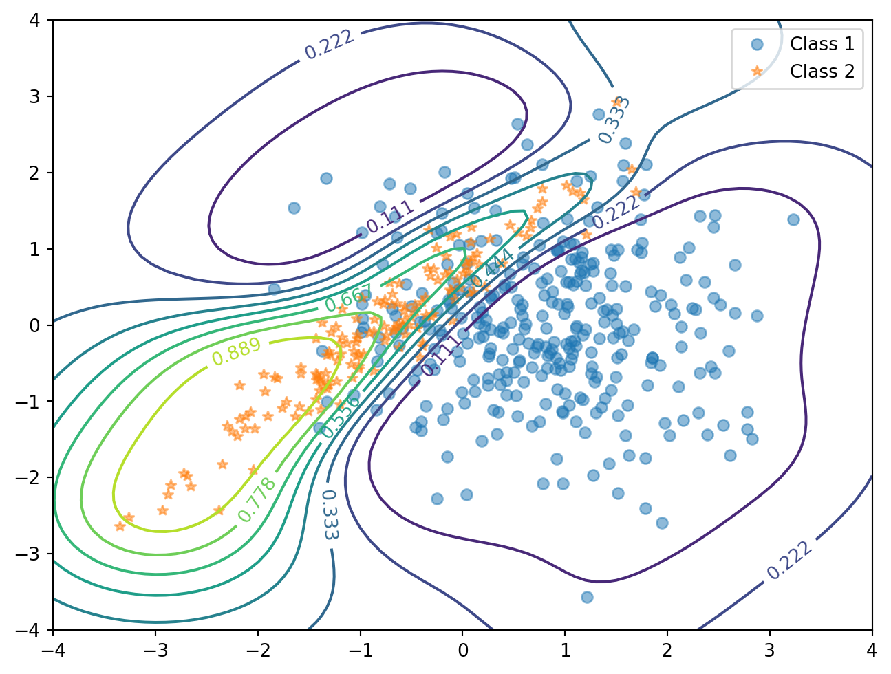
類似度行列 \(W\) に関して，確率的近傍埋め込み でも使うモデル \[ p_{ij}^W:=\frac{\exp\left(-\lvert Wx_i-Wx_j\rvert^2\right)}{\sum_{k\neq i}\exp\left(-\lvert Wx_i-Wx_k\rvert^2\right)} \] を考える．各 \(i\in[n]\) について，\(x_i\) 以外のデータから \(x_j\) のラベルを \(1\)-近傍分類器で正しく予測する確率が最大になるように， \[ \mathcal{L}(W):=1-\frac{1}{N}J(W),\quad J(W):=\sum_{i=1}^n\sum_{(i,j)\in E}p_{ij}^W \] を最小化するように学習する．ただし，辺の集合 \(E\) は，ラベルの同じデータを結ぶとした．

2.4 深層距離学習

2.4.1 分類に基づく目的関数

深層距離学習では目的関数の設定が重要である．

最も初等的には，自己符号化器などで分類問題を解き，その内部表現（よく最後から２層目を用いる）での Euclid 距離を距離関数に用いる方法がある．

しかし，距離の情報を学習するために，分類タスクは弱すぎるようである．

2.4.2 ２者比較に基づく目的関数

\[ \mathcal{L}(\theta;x_i,x_j):=\delta_{y_i,y_j}d(z_i,z_j)^2+(1-\delta_{y_i,y_j})\biggr(m-d(z_i,z_j)^2\biggl)_+,\qquad z_i=f_\theta(x_i) \] という損失関数は 対照的損失 (contrastive loss) (Chopra et al., 2005) と呼ばれる．

この損失はラベル \(y_i,y_j\) が同一のデータ \(x_i,x_j\) の潜在表現の距離を近づけ，ラベルが異なるデータは \(m\) 以上は話すように埋め込み \(f_\theta\) を学習する．

この際に用いるニューラルネットワークは，同時に２つの入力 \(x_i,x_j\) をとって学習することから，双子ネットワーク (Siamese network) とも呼ばれる．

2.4.3 ３者比較に基づく目的関数

この方法は直ちに三子損失 (triplet loss) (Schroff et al., 2015)，\(n\)-ペア損失 (\(n\)-pair loss) (Sohn, 2016), (Oord et al., 2018) に拡張された．

このことにより，\(x_i,x_j\) の「近さ」のスケールと「遠さ」のスケールが一致し，安定した結果が得られる．

三子損失は，各データ \(x_i\) に対して，「似ている」ペア \(x_i^+\) と「似ていない」ペア \(x_i^-\) を事前に選び， \[ \mathcal{L}(\theta;x_i,x_i^+,x_i^-):=\biggr(d_\theta(x_i,x_i^+)^2-d_\theta(x_i,x_i^-)^2+m\biggl)_+,\qquad m\in\mathbb{R} \] と定められる．このとき，\(x_i\) は参照点 (anchor) と呼ばれる．

この方法は \(x_i^+,x_i^-\) を選ばなければいけないが，その分拡張性に優れる．ノイズ対照学習 の稿も参照．

\(n\)-ペア損失では，負のデータ \(x_i^-\) をさらに増やす．これは (Oord et al., 2019 Contrastive Predictive Coding) にて，InfoMax の観点から表現学習に用いられたものと一致する．

2.4.4 ３者比較の加速

負の例 \(x_i^-\) を特に情報量が高いもの (hard negatives, Faghri et al., 2018) を選ぶことで，学習を加速させることができる．

これは，３者損失を提案した Google の FaceNet (Schroff et al., 2015) で考えられた戦略である．

クラスラベルが得られる場合，各クラスから代表的なデータを選んでおくことで \(O(n)\) にまで加速できる (Movshovitz-Attias et al., 2017)．この代表点は固定して１つに定める必要はなく，ソフトな形で選べる (Qian et al., 2019)．

3 終わりに

ここで扱った深層距離学習は，現代的には表現学習として更なる発展を見ている．

References

Borgwardt, K., Schraudolph, N., and Vishwanathan, S. v. n. (2006). Fast computation of graph kernels. In B. Schölkopf, J. Platt, and T. Hoffman, editors, Advances in neural information processing systems,Vol. 19. MIT Press.

Chaudhuri, K., and Dasgupta, S. (2014). Rates of convergence for nearest neighbor classification. In Z. Ghahramani, M. Welling, C. Cortes, N. Lawrence, and K. Q. Weinberger, editors, Advances in neural information processing systems,Vol. 27. Curran Associates, Inc.

Chopra, S., Hadsell, R., and LeCun, Y. (2005). Learning a similarity metric discriminatively, with application to face verification. 2005 IEEE Computer Society Conference on Computer Vision and Pattern Recognition (CVPR’05), 1, 539–546.

Cleveland, W. S. (1979). Robust locally weighted regression and smoothing scatterplots. Journal of the American Statistical Association, 74(368), 829–836.

Cleveland, W. S., and Devlin, S. J. (1988). Locally weighted regression: An approach to regression analysis by local fitting. Journal of the American Statistical Association, 83(403), 596–610.

Faghri, F., Fleet, D. J., Kiros, J. R., and Fidler, S. (2018). VSE++: Improving visual-semantic embeddings with hard negatives.

Gibbs, M. N. (1997). Bayesian gaussian process regression and classification (PhD thesis). Cambridge University. Retrieved from https://citeseerx.ist.psu.edu/document?repid=rep1&type=pdf&doi=b5a0c62c8d7cf51137bfb079947b8393c00ed169

Goldberger, J., Hinton, G. E., Roweis, S., and Salakhutdinov, R. R. (2004). Neighbourhood components analysis. In L. Saul, Y. Weiss, and L. Bottou, editors, Advances in neural information processing systems,Vol. 17. MIT Press.

Heinonen, M., Mannerström, H., Rousu, J., Kaski, S., and Lähdesmäki, H. (2016). Non-stationary gaussian process regression with hamiltonian monte carlo. In A. Gretton and C. C. Robert, editors, Proceedings of the 19th international conference on artificial intelligence and statistics,Vol. 51, pages 732–740. Cadiz, Spain: PMLR.

Jona-Lasinio, G., Gelfand, A., and Jona-Lasinio, M. (2012). SPATIAL ANALYSIS OF WAVE DIRECTION DATA USING WRAPPED GAUSSIAN PROCESSES. The Annals of Applied Statistics, 6(4), 1478–1498.

Kriege, N. M., Johansson, F. D., and Morris, C. (2020). A survey on graph kernels. Applied Network Science, 5(1), 6.

Liu, H., Ong, Y.-S., Shen, X., and Cai, J. (2020). When gaussian process meets big data: A review of scalable GPs. IEEE Transactions on Neural Networks and Learning Systems, 31(11), 4405–4423.

Lloyd, S. (1982). Least squares quantization in PCM. IEEE Transactions on Information Theory, 28(2), 129–137.

Lodhi, H., Saunders, C., Shawe-Taylor, J., Cristianini, N., and Watkins, C. (2002). Text classification using string kernels. Journal of Machine Learning Research, 2, 419–444.

Loeliger, H.-A., Bruderer, L., Malmberg, H., Wadehn, F., and Zalmai, N. (2016). On sparsity by NUV-EM, gaussian message passing, and kalman smoothing. In 2016 information theory and applications workshop (ITA), pages 1–10.

MacKay, D. J. C. (1994). Bayesian nonlinear modeling for the prediction competition (No. 2),Vol. 100. American Society of Heating, Refrigerating,; Air Conditioning Engineers (ASHRAE). Retrieved from https://www.osti.gov/biblio/33309

MacQueen, J. (1967). Some methods for classification and analysis of multivariate observations. In Proceedings of the fifth berkeley symposium on mathematical statistics and probability,Vol. 1, pages 281–297.

Movshovitz-Attias, Y., Toshev, A., Leung, T. K., Ioffe, S., and Singh, S. (2017). No fuss distance metric learning using proxies. In 2017 IEEE international conference on computer vision (ICCV), pages 360–368. Los Alamitos, CA, USA: IEEE Computer Society.

Murphy, K. P. (2022). Probabilistic machine learning: An introduction. MIT Press.

Murphy, K. P. (2023). Probabilistic machine learning: Advanced topics. MIT Press.

Musgrave, K., Belongie, S., and Lim, S.-N. (2020). A metric learning reality check. In A. Vedaldi, H. Bischof, T. Brox, and J.-M. Frahm, editors, Computer vision – ECCV 2020, pages 681–699. Cham: Springer International Publishing.

Nadaraya, E. A. (1964). On estimating regression. Theory of Probability & Its Applications, 9(1), 141–142.

Neal, R. M. (1996). Bayesian learning for neural networks,Vol. 118. Springer New York.

Oord, A. van den, Li, Y., Babuschkin, I., Simonyan, K., Vinyals, O., Kavukcuoglu, K., … Hassabis, D. (2018). Parallel WaveNet: Fast high-fidelity speech synthesis. In J. Dy and A. Krause, editors, Proceedings of the 35th international conference on machine learning,Vol. 80, pages 3918–3926. PMLR.

Oord, A. van den, Li, Y., and Vinyals, O. (2019). Representation learning with contrastive predictive coding.

Qian, Q., Shang, L., Sun, B., Hu, J., Li, H., and Jin, R. (2019). SoftTriple loss: Deep metric learning without triplet sampling. In Proceedings of the IEEE/CVF international conference on computer vision (ICCV).

Rahimi, A., and Recht, B. (2007). Random features for large-scale kernel machines. In J. Platt, D. Koller, Y. Singer, and S. Roweis, editors, Advances in neural information processing systems,Vol. 20. Curran Associates, Inc.

Rahimi, A., and Recht, B. (2008). Weighted sums of random kitchen sinks: Replacing minimization with randomization in learning. In D. Koller, D. Schuurmans, Y. Bengio, and L. Bottou, editors, Advances in neural information processing systems,Vol. 21. Curran Associates, Inc.

Rasmussen, C. E., and Williams, C. K. I. (2006). Gaussian processes for machine learning. The MIT Press.

Remes, S., Heinonen, M., and Kaski, S. (2017). Non-stationary spectral kernels. In I. Guyon, U. V. Luxburg, S. Bengio, H. Wallach, R. Fergus, S. Vishwanathan, and R. Garnett, editors, Advances in neural information processing systems,Vol. 30. Curran Associates, Inc.

Savitzky, Abraham., and Golay, M. J. E. (1964). Smoothing and differentiation of data by simplified least squares procedures. Analytical Chemistry, 36(8), 1627–1639. doi: 10.1021/ac60214a047.

Schroff, F., Kalenichenko, D., and Philbin, J. (2015). FaceNet: A unified embedding for face recognition and clustering. In Proceedings of the IEEE conference on computer vision and pattern recognition (CVPR).

Shervashidze, N., Schweitzer, P., Leeuwen, E. J. van, Mehlhorn, K., and Borgwardt, K. M. (2011). Weisfeiler-lehman graph kernels. Journal of Machine Learning Research, 12(77), 2539–2561.

Sohn, K. (2016). Improved deep metric learning with multi-class n-pair loss objective. In D. Lee, M. Sugiyama, U. Luxburg, I. Guyon, and R. Garnett, editors, Advances in neural information processing systems,Vol. 29. Curran Associates, Inc.

Sutherland, D. J., and Schneider, J. (2015). On the error of random fourier features. In Proceedings of the thirty-first conference on uncertainty in artificial intelligence, pages 862–871. Arlington, Virginia, USA: AUAI Press.

Tipping, M. E. (2001). Sparse bayesian learning and the relevance vector machine. Journal of Machine Learning Research, 1, 211–244.

Watson, G. S. (1964). Smooth regression analysis. Sankhyā: The Indian Journal of Statistics, Series A (1961-2002), 26(4), 359–372.

Weinberger, Kilian Q., Blitzer, J., and Saul, L. (2005). Distance metric learning for large margin nearest neighbor classification. In Y. Weiss, B. Schölkopf, and J. Platt, editors, Advances in neural information processing systems,Vol. 18. MIT Press.

Weinberger, Kilian Q., and Saul, L. K. (2009). Distance metric learning for large margin nearest neighbor classification. Journal of Machine Learning Research, 10(9), 207–244.

Wilson, A., and Adams, R. (2013). Gaussian process kernels for pattern discovery and extrapolation. In S. Dasgupta and D. McAllester, editors, Proceedings of the 30th international conference on machine learning,Vol. 28, pages 1067–1075. Atlanta, Georgia, USA: PMLR.

Yu, F. X. X., Suresh, A. T., Choromanski, K. M., Holtmann-Rice, D. N., and Kumar, S. (2016). Orthogonal random features. In D. Lee, M. Sugiyama, U. Luxburg, I. Guyon, and R. Garnett, editors, Advances in neural information processing systems,Vol. 29. Curran Associates, Inc.

持橋大地, and 大羽成征. (2019). ガウス過程と機械学習. 講談社.

Footnotes

1. (Murphy, 2022, p. 565) 17.1節は，半正定値核のことを Mercer 核とも呼んでいる．

2. RBF は (持橋大地 and 大羽成征, 2019, p. 68)，SE は (Rasmussen and Williams, 2006, p. 14) の用語．(Murphy, 2023) では両方が併記されている．Gaussian kernel とも呼ばれる．

3. 他のパラメータの入れ方もある．例えば GPy での実装 は \(\sigma^2\exp\left(-\frac{r^2}{2}\right)\) を採用している．Fourier 変換や偏微分方程式論の文脈では \(\frac{1}{(4\pi t)^{d/2}}\exp\left(-\frac{r^2}{4}\right)\) も良く用いられる．これは熱方程式の基本解になるためである．

4. (MacKay, 1994), (Neal, 1996, p. 16) なども参照．