概要

生成・表現学習と深い関係にあるタスクに，次元縮約がある．非線型な次元縮約法は多様体学習の名前の下でも研究されている．表現学習とも関連が深いが，一般に表現学習はパラメトリックであるとするならば，次元縮約ではノンパラメトリックな表現と視覚化の学習が目標である．

1 はじめに

多様体学習とは，非線型な次元削減手法のことをいう．

1.1 多様体仮説

「多様体」の名前の由来は，「高次元データは低次元の部分多様体としての構造を持つ」という 多様体仮説 (Fefferman et al., 2016) である．¹

特に多様体学習と呼ばれる際は，知識発見やデータ可視化を重視する志向がある．

一方で自己符号化器などによる表現学習では，種々の下流タスクに有用な表現を得るための分布外汎化が重視される，と言えるだろう．

1.2 距離学習との関係

近年，対照学習による表現学習が注目されている．このアプローチには，目的関数にサンプル間の類似度に関する事前情報を含めやすいという美点がある．

このような表現学習法は 距離学習 (metric learning) とも呼ばれている．

多くの多様体学習手法や，\(\mathbb{R}^d\) への埋め込み手法は，なんらかの意味でサンプル間の類似度を保存する埋め込みを求めている (Agrawal et al., 2021)．

この意味で，「距離学習」というキーワードは，表現学習と多様体学習の交差点を意味していると言えるだろう．

1.3 例：細胞間の類似度

現代のシークエンサー NGS (Next Generation Sequencer) では，単一の細胞が保持している mRNA の全体 scRNA-seq (single-cell RNA sequencing) を調べることができ，このような場合は極めて高次元のデータが大量に得られることになる．

例えば COVID-19 重症患者の末梢免疫の状態を調べるために末梢血単核細胞 PBMC² から scRNA-seq を行った例 (Wilk et al., 2020) では，全部で \(n=44,721\) の細胞のデータが，\(p=26361\) 次元のスパースなベクトルを扱っている．³

2 多次元尺度法 (MDS)

2.1 概要

多次元尺度法 (MDS: Multi-Dimensional Scaling) (Torgerson, 1952), (Kruskal, 1964) は，元のデータの「（非）類似度」を保存したままの低次元表現を探索する手法群である．

後続の手法はいずれも高次元データ \(\{y_i\}_{i=1}^n\subset\mathbb{R}^p\) を所与とするが，MDS は本質的には類似度行列 \(D\in M_n(\mathbb{R})\) が与えられていればよく，解析対象は必ずしも \(\mathbb{R}^p\)-値のデータである必要はない．

類似度行列 \(D\) が与えられたのちは，埋め込み \(\{z_i\}_{i=1}^n\subset\mathbb{R}^d\) の要素間の類似度が \(D\) に近くなるように埋め込みを学習する．

2.2 PCA としての MDS

特にデータ \(\{x_i\}_{i=1}^n\subset\mathbb{R}^p\) 間の Euclid 距離を \(D\) とし，埋め込み \(\{z_i\}_{i=1}^n\subset\mathbb{R}^d\) の間の経験共分散が \(D\) に Hilbert-Schmidt ノルムに関して最小化することを (Torgerson, 1952) は考えた．

これは (Eckart and Young, 1936) の定理を通じて PCA に一致する，線型な次元縮約法となる．

(Torgerson, 1952) のアプローチは計量多次元尺度法と呼ばれ，一般のデータに適用可能な (Kruskal, 1964) のアプローチは非計量多次元尺度法と対照される．⁴

2.3 (Kruskal, 1964) Stress

前述の通り，\(D\) は Euclid 距離に基づくとは限らないし，そもそもデータはベクトルなど構造化されているものでなくても良い．

このような一般的な場面で \(\{z_i\}_{i=1}^n\subset\mathbb{R}^d\) 間の類似度の \(D\) との「近さ」を図る尺度として，Kruskal の Stress-1 (Kruskal, 1964) がよく用いられる： \[ \mathcal{L}(E):=\sqrt{\frac{\sum_{i_1<i_2}\left(z_{i_1i_2}-d_{i_1i_2}\right)^2}{\sum_{i_1<i_2}d_{i_1i_2}^2}}. \]

勾配法を用いた最適化ベースの推論手法が使えるが，この目的関数に関しては SMACOF (Scaling by Majorizing a Complementary Function) (de Leeuw, 1977) という凸最適化アルゴリズムが提案されており，scikit-learn にも実装されている．

2.4 (Sammon, 1969) Stress

(Sammon, 1969) は探索的データ解析の文脈から，データの「構造」をよく保つために，\(z_{i_1i_2}\) の値が小さい場合は小さな変化も重視してくれるようにスケーリングを調整する新たなストレス関数を提案した：

\[ \frac{1}{\sum_{i_1<i_2}z_{i_1i_2}}\sum_{i_1<i_2}\frac{\left(z_{i_1i_2}-d_{i_1i_2}\right)^2}{z_{i_1i_2}}. \]

係数 \(\frac{1}{\sum_{i_1<i_2}z_{i_1i_2}}\) の存在は，勾配法による推論を効率的にする．

2.5 多次元展開法 (MDU)

多次元展開法 (MDU: Multi-Dimensional Unfolding) は，個人の選考順位データに対処するために (Coombs, 1950) が提唱した，多次元尺度法 (MDS) の拡張である (足立浩平, 2000)．

MDU ではさらに一般的な行列 \(D\) を取ることができる．というのも，MDS では暗黙のうちに行と列は同一物であり，\(D\) の対角成分は全て一定であるが，MDU では行と列で別の対象を取ることができる．

例えば，個体 \(i\) が項目 \(j\) をどれくらい好むか？を \(D\) と取り，行と列を同一の平面上にバイプロット (Gabriel, 1971), (Gower, 2004) する．

2.6 理想点推定

特に政治科学の分野で用いられる多次元展開手法であり，\(\mathbb{R}^d\;(d\le3)\) に埋め込むことが考えられる．

その際は \(\mathbb{R}^d\) 上への観測に至るまでの階層モデル（潜在変数モデル）を立てて，全体を MCMC により推定する方法が，(Martin and Quinn, 2002) 以来中心的である．

(Imai et al., 2016)，(三輪洋文, 2017) は変分 EM アルゴリズムにより推定している．

2.7 力指向グラフ展開 (FDL / SE)

力学モデルによるグラフ描画法 (Force-directed layout / Spring Embedder) (Tutte, 1963), (Eades, 1984), (Kamada and Kawai, 1989) は，グラフの頂点を質点，辺をバネに見立てて，グラフを \(\mathbb{R}^2\) 上に展開する方法である．

超大規模集積回路 (VLSI) の設計問題と両輪で発展してきた (Fisk et al., 1967), (Quinn and Breuer, 1979)．

このグラフ埋め込み法はポテンシャルエネルギーをストレスと見立てた MDS とみなせる．

3 Isomap

MDS 法の難点の１つに，データがある部分多様体上に存在する場合，その部分多様体上の測地距離を尊重できないという点がある．

このデータの部分多様体構造を尊重した測地距離をグラフにより捉え，MDS を実行する手法が Isomap (Tenenbaum et al., 2000) である．

Isomap：データの多様体構造を尊重した MDS

データを頂点とした \(K\)-近傍グラフを構成する．
測地距離を，このグラフ上の最短距離として近似する．
こうして得た近似測地距離を用いて MDS を行う．

ステップ２においては Dijkstra 法を用いることができ，高速な計算が可能である．

しかし Isomap はデータの摂動に極めて弱いことが topological instability として知られている (Balasubramanian and Schwartz, 2002)．

この安定性をカーネル法に外注する Robust Kernel Isomap (Choi and Choi, 2007) も提案されている．

4 最大分散展開 (MVU)

4.1 カーネル PCA (kPCA) (Schölkopf et al., 1998)

カーネル法の見地からは，従来の PCA は線型な核を用いた場合のカーネル主成分分析だったと相対化される．

しかし，少なくとも RBF カーネルを用いた場合は (Weinberger et al., 2004)，次元縮約の代わりにより高次元な空間に埋め込みがちである．

4.2 半正定値埋め込み

カーネル PCA を次元縮約のために用いたものが 半正定値埋め込み (semidefinite embedding) または 最大分散展開 (MVU: Maximum Vairance Unfolding) (Weinberger et al., 2004) である．

これは，カーネル PCA による埋め込みの中でも，元データ \(y\) と埋め込み \(z\) の間で \[ \|z_i-z_j\|_2=\|y_i-y_j\|_2,\qquad(i,j)\in G \] を \(K\)-近傍 \(G\) に関して満たすような埋め込みの中で， \[ \max_{z\in\mathbb{R}^d}\sum_{i,j}\|z_i-z_j\|_2^2 \] を最大にするものを求めることを考える．

幸い，これを満たすカーネル関数は半正定値計画によって解くことができ，このカーネル関数によるカーネル PCA 法が MVU である．

5 局所線型埋め込み (LLE)

5.1 はじめに

ここまでの手法は畢竟，類似度行列 \(Y\) に関して，kPCA は特徴空間上でのスペクトル分解，Isomap はデータのなす \(K\)-近傍グラフ上でのスペクトル分解を考えている．

これに対して，スパースなスペクトル分解を用いることで，データの局所的構造がさらに尊重できることが，局所線型埋め込み (LLE: Local Linear Embedding) (Roweis and Saul, 2000) として提案された．

この方法は Isomap よりデータの摂動に関して頑健であることが知られている．

5.2 アルゴリズム

この方法では，データ多様体の接空間に注目する．

まず，各点をその \(K\)-近傍点の線型結合で表す方法を，次のように学習する： \[ \widehat{W}=\min_{W}\sum_{i=1}^n\left(x_i-\sum_{j=1}^nw_{ij}x_j\right)^2,\qquad\operatorname{subject to}\begin{cases}w_{ij}=0&x_i,x_j\,\text{は}\,K\text{-近傍でない}\\\sum_{j=1}^Nw_{ij}=1&\text{任意の}\,i\in[N]\,\text{について}\end{cases} \] こうして得た \(\widehat{W}\) はスパース行列になる．この \(W\) を通じて，局所構造を保った低次元埋め込みを構成する： \[ \widehat{Z}=\operatorname*{argmin}_Z\sum_{i=1}^n\left\|z_i-\sum_{j=1}^n\widehat{w}_{ij}z_j\right\|_2^2. \]

この最適化問題は，\(I_n-W\) の特異値分解に帰着する．

5.3 Hessian 埋め込み (HE)

Hessian Eigenmaps (Donoho and Grimes, 2003) は微分幾何学的見方を推し進め，Hessian からの情報を取り入れた局所線型埋め込みの変種である．

5.4 接空間配置 (TSA)

Tangent Space Alignment (Zhang and Zha, 2004) はより明示的に接空間の構造に注目する．

6 スペクトル埋め込み (SE / LE)

Laplacian Eigenmaps または Spectral Embedding (Belkin and Niyogi, 2001) は，データ点の \(K\)-近傍グラフ \((Y,E)\) 上で \[ \mathcal{L}(Z):=\sum_{(i,j)\in E}W_{ij}\|z_i-z_j\|_2^2,\qquad W_{ij}:=\exp\left(-\frac{\|y_i-y_j\|_2^2}{2\sigma^2}\right) \] を最小化する埋め込み \(Z\) を求める方法である．

この目的関数 \(\mathcal{L}(Z)\) は実は，\(K\)-近傍グラフ \((Y,E)\) の Laplacian 行列 \(L\) に関して \[ \mathcal{L}(Z)=2\operatorname{Tr}(Z^\top LZ) \] とも表せる．

この量は，\(Z\) をグラフ上の関数と見た際の Dirichlet 汎函数になっており，グラフ上の関数としての「滑らかさ」の尺度となっている．

最も滑らかであるような \(Z\) を学習することで，データの局所構造を最も反映した埋め込みが得られる，というアイデアである．

7 \(t\)-分布型確率的近傍埋め込み (t-SNE)

7.1 概要

SNE (Hinton and Roweis, 2002) では，\(K\)-近傍グラフを用いた Isomap を，ハードな帰属からソフトな帰属へ，確率分布を用いて軟化する．

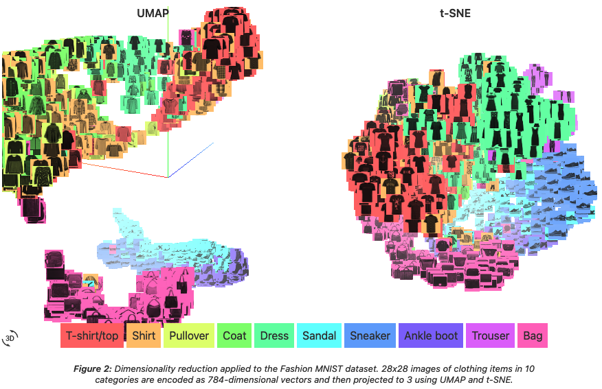
t-SNE (van der Maaten and Hinton, 2008) では SNE が Gauss 核を用いていたところを Laplace 核（\(t\)-分布）を用いることで，より分散した表現を得ることを目指す．

7.2 確率的近傍埋め込み (SNE, Hinton and Roweis, 2002)

ハイパーパラメータ \(\sigma_i\) を残して， \[ p_{j|i}:=\frac{\exp\left(-\frac{\lvert x_i-x_j\rvert^2}{2\sigma_i^2}\right)}{\sum_{k\neq i}\exp\left(-\frac{\lvert x_i-x_k\rvert^2}{2\sigma_i^2}\right)} \] と定める．

この \((p_{j|i})\) と，潜在空間における帰属確率 \[ q_{j|i}:=\frac{e^{-\lvert z_i-z_j\rvert^2}}{\sum_{k\neq i}e^{-\lvert z_i-z_k\rvert^2}} \] と一致するように埋め込みを学習する．すなわち，訓練目標は \[ \mathcal{L}:=\sum_{i=1}^n\operatorname{KL}(p_{-|i},q_{-|i})=\sum_{i,j=1}^np_{j|i}\log\frac{p_{j|i}}{q_{j|i}} \] と定める．

この目的関数は凸ではなく，SGD で訓練可能であるが特殊なノイズスケジュールなどのテクニックがある．⁵

SNE は，ある事前分布を課したスペクトル埋め込みとも見れる (Carreira-Perpiñan, 2010)．

7.3 目的関数の対称化

\(p_{i|j},q_{i|j}\) ではなく，結合分布 \(p_{ij},q_{ij}\) を用いることで，目的関数を対称化することができる．

このとき，目的関数の勾配は次のようになる： \[ \nabla_{z_i}\mathcal{L}(Z)=2\sum_{j=1}^n(z_j-z_i)(p_{ij}-q_{ij}). \]

7.4 \(t\)-分布の導入

t-SNE (van der Maaten and Hinton, 2008) は \(p_{j|i}\) の定義に Gauss 核を用いていたところを，Cauchy 分布の密度（Poisson 核）に置き換えたものである： \[ q_{ij}=\frac{\frac{1}{1+\lvert z_i-z_j\rvert^2}}{\sum_{k<l}\frac{1}{1+\lvert z_k-z_l\rvert^2}}. \]

このことにより，元々遠かったデータ点を引き寄せ過ぎてしまうこと (crowding problem) を回避できる．

勾配は \[ \nabla_{z_i}\mathcal{L}(Z)=4\sum_{j=1}^n(z_j-z_i)(p_{ij}-q_{ij})\frac{1}{1+\lvert z_i-z_j\rvert^2} \] で与えられ，対称化された SNE に，\(z_i,z_j\) の距離に従って調整する因子が追加された形になっている．

7.5 実装

t-SNE は \(O(n^2)\) であるが，埋め込みの次元数が \(d=2\) などの低次元であるとき，これを \(O(n\log n)\) にまで加速する実装が知られている (Maaten, 2014)．

7.6 敏捷な埋め込み (EE)

t-SNE はハイパーパラメータ \(\sigma_i^2\) の設定に敏感である上に訓練が局所解にトラップされるなど不安定で，またデータ内のノイズに弱いことが知られている (Wattenberg et al., 2016)．

敏捷な埋め込み (EN: Elastic Net) (Carreira-Perpiñan, 2010) という，より安定的でノイズに頑健な手法が目的関数を修正することで得られている．

7.7 LargeVis

LargeVis (Tang et al., 2016) は t-SNE の計算量を軽減させるために，\(K\)-近傍グラフの計算に近似手法である ランダム射影木 (Dasgupta and Freund, 2008) を導入する．

7.8 UMAP

UMAP (Uniform Manifold Approximation and Projection) (McInnes et al., 2018) は t-SNE より高速で，大域的構造をより尊重する手法として提案された．

UMAP and t-SNE applied to the Fashion MNIST dataset; tap to visit https://pair-code.github.io/understanding-umap/

7.9 モデルベース手法

t-SNE, VargeVis, UMAP はいずれも確率を導入しているが，完全にモデルベースの発想をしているわけではない．

(Saul, 2020) はこれらの手法を潜在変数モデルとして定式化し，データサイズに合わせて EM アルゴリズムをはじめとした推定手法を議論している．

8 拡散写像

8.1 はじめに

拡散埋め込み (Diffusion Map) (Coifman et al., 2005) では，データ上に乱歩を定めることでデータ多様体の局所構造を捉える．

この方法は Isomap 3 でグラフを用いて測地距離を近似したよりも，頑健なアルゴリズムを与える．

8.2 PHATE

PHATE (Heat Diffusion for Affinity-based Transition Embedding) (Moon et al., 2019) は DEMaP (Denoised Embedding Manifold Preservation) という情報理論に基づく距離を定義し，データの局所構造を捉える．

9 自己組織化写像 (SOM)

Self-organizing Map (Kohonen, 1982), (Kohonen, 2013) は，ニューラルネットワークのダイナミクスを利用した，クラスタリングベースの次元縮約法である．

9.1 IVIS

IVIS (Szubert et al., 2019) は三つ子損失を取り入れたシャムネットワークによる距離学習に基づく次元縮約法である．

10 Mapper

Mapper (Singh et al., 2007) は，距離空間 \(E\) 上のデータ \(\{x_i\}\subset E\) を，関数 \(f:E\to\mathbb{R}\) が定める分解を用いてグラフとして図示する方法である．\(f\) は filter function と呼ばれる．

他手法とは違い，出力が \(\mathbb{R}^d\) への埋め込みではなく，グラフである点に注意．

Mapper アルゴリズム⁶

値の空間 \(\mathbb{R}\) 上の開被覆 \((I_i)\) の引き戻し \(\mathcal{U}:=(f^{-1}(I_i))\) として誘導されるグラフを，連結成分のみからなるように細分して \(\mathcal{V}=(U_i)_{i\in I}\) を得る．
\(\mathcal{V}\) の神経複体 \[ N(\mathcal{V}):=\left\{J\overset{\text{finite}}{\subset}I\,\middle|\,\bigcap_{j\in J}U_j\ne\emptyset\right\} \] またはその近傍グラフを出力とする．

(Escolar et al., 2023) では特許のデータを用い，各企業を技術空間 \(\mathbb{R}^{430}\) 内に埋め込んだ後，mapper によりグラフ化したところ，企業の独自戦略が可視化できるという：

Mapper アルゴリズムは filter function \(f\) の選択が重要になるが，これにハイパーパラメータを導入し (Oulhaj, Carrière, et al., 2024)，さらにニューラルネットワークで推定する方法 Deep Mapper (Oulhaj, Ishii, et al., 2024) が，分子モデリングと創薬に応用されている．

11 終わりに

結局機械学習が日々の統計的営みに与えた最大のインパクトは，ニューラルネットワークや生成モデル自体というより，高精度な非線型表現学習であると言えるかもしれない．

例えば (Hoffman et al., 2019) は IAF (Kingma et al., 2016) を用いて目標分布を学習し，学習された密度 \(q\) で変換後の分布から MCMC サンプリングをすることで効率がはるかに改善することを報告した．実際，フローによる変換を受けた後は対象分布は正規分布に近くなることから，MCMC サンプリングを減速させる要因の多くが消滅していることが期待される．

多くの他の統計的な困難も，良い表現学習された空間上（あるいはカーネル空間上）で実行することで回避することができるということになるかもしれない．これが最初に SVM が機械学習に与えた希望の形であったし，ニューラルネットワークに対する飽くなき理論的興味の源泉でもある．データの視覚化や探索的データ解析の意味では，よき潜在表現を必要としているのは人間も然りである．

12 文献

(Yao, 2011) は LLE, Laplacian Eigenmaps, カーネル PCA, Diffusion Maps の関連性を扱っている講義スライドである．

(Wattenberg et al., 2016) はインタラクティブに t-SNE の性質を理解できるウェブページである．Understanding UMAP も同様にして，UMAP と t-SNE の比較を与えている．

(Murphy, 2022) 第20章は次元縮約という題で，PCA, FA から自己符号化器，多様体学習を解説している．(Burges, 2010) が同じテーマのしばらく前のサーベイである．

多様体学習に関しては (本武陽一, 2017) も注目．

PCA は Kosambi-Karhunen-Loéve 変換ともいう (Bishop and Bishop, 2024, p. 497)．PCA からとにかくスペクトルとの関連が深い．

References

Agrawal, A., Ali, A., and Boyd, S. (2021). Minimum-distortion embedding. Foundations and Trends in Machine Learning, 14(3), 211–378.

Balasubramanian, M., and Schwartz, E. L. (2002). The isomap algorithm and topological stability. Science, 295(5552), 7–7.

Belkin, M., and Niyogi, P. (2001). Laplacian eigenmaps and spectral techniques for embedding and clustering. In T. Dietterich, S. Becker, and Z. Ghahramani, editors, Advances in neural information processing systems,Vol. 14. MIT Press.

Bishop, C. M., and Bishop, H. (2024). Deep learning: Foundations and concepts. Springer Cham.

Burges, C. J. C. (2010). Dimension reduction: A guided tour. Foundations and Trends in Machine Learning, 2(4), 275–365.

Carreira-Perpiñan, M. Á. (2010). The elastic embedding algorithm for dimensionality reduction. In Proceedings of the 27th international conference on international conference on machine learning, pages 167–174. Madison, WI, USA: Omnipress.

Choi, H., and Choi, S. (2007). Robust kernel isomap. Pattern Recognition, 40(3), 853–862.

Coifman, R. R., Lafon, S., Lee, A. B., Maggioni, M., Nadler, B., Warner, F., and Zucker, S. W. (2005). Geometric diffusions as a tool for harmonic analysis and structure definition of data: Diffusion maps. Proceedings of the National Academy of Sciences, 102(21), 7426–7431.

Coombs, C. H. (1950). Psychological Scaling without a Unit of Measurement. Psychological Review, 57(3), 145–158.

Dasgupta, S., and Freund, Y. (2008). Random projection trees and low dimensional manifolds. In Proceedings of the fortieth annual ACM symposium on theory of computing, pages 537–546. New York, NY, USA: Association for Computing Machinery.

de Leeuw, J. (1977). Applications of convex analysis to multidimensional scaling. UCLA: Department of Statistics. Retrieved from https://escholarship.org/uc/item/7wg0k7xq

Donoho, D. L., and Grimes, C. (2003). Hessian eigenmaps: Locally linear embedding techniques for high-dimensional data. Proceedings of the National Academy of Sciences, 100(10), 5591–5596.

Eades, P. (1984). A Heuristic for Graph Drawing. Congress Numerantium, 42(11), 149–160.

Eckart, C., and Young, G. (1936). The approximation of one matrix by another of lower rank. Psychometrika, 1(3), 211–218.

Escolar, E. G., Hiraoka, Y., Igami, M., and Ozcan, Y. (2023). Mapping firms’ locations in technological space: A topological analysis of patent statistics. Research Policy, 52(8), 104821.

Fefferman, C., Mitter, S., and Narayanan, H. (2016). Testing the manifold hypothesis. Journal of the American Mathematical Society, 29, 983–1049.

Fisk, C. J., Caskey, D. L., and West, L. E. (1967). ACCEL: Automated circuit card etching layout. Proceedings of the IEEE, 55(11), 1971–1982.

Gabriel, K. R. (1971). The biplot graphic display of matrices with application to principal component analysis. Biometrika, 58(3), 453–467.

Gower, J. C. (2004). The geometry of biplot scaling. Biometrika, 91(3), 705–714.

Hinton, G. E., and Roweis, S. (2002). Stochastic neighbor embedding. In S. Becker, S. Thrun, and K. Obermayer, editors, Advances in neural information processing systems,Vol. 15. MIT Press.

Hoffman, M., Sountsov, P., Dillon, J. V., Langmore, I., Tran, D., and Vasudevan, S. (2019). NeuTra-lizing bad geometry in hamiltonian monte carlo using neural transport. In Symposium on advances in approximate bayesian inference.

Imai, K., Lo, J., and Olmsted, J. (2016). Fast Estimation of Ideal Points with Massive Data. American Political Science Review, 110(4), 631–656.

Kamada, T., and Kawai, S. (1989). An algorithm for drawing general undirected graphs. Information Processing Letters, 31(1), 7–15.

Kingma, D., Salimans, T., Jozefowicz, R., Chen, X., Sutskever, I., and Welling, M. (2016). Improved variational inference with inverse autoregressive flow. In D. Lee, M. Sugiyama, U. Luxburg, I. Guyon, and R. Garnett, editors, Advances in neural information processing systems,Vol. 29. Curran Associates, Inc.

Kohonen, T. (1982). Self-organized formation of topologically correct feature maps. Biological Cybernetics, 43(1), 59–69.

Kohonen, T. (2013). Essentials of the self-organizing map. Neural Networks, 37, 52–65.

Kruskal, J. B. (1964). Multidimensional scaling by optimizing goodness of fit to a nonmetric hypothesis. Psychometrika, 29(1), 1–27.

Maaten, L. van der. (2014). Accelerating t-SNE using tree-based algorithms. Journal of Machine Learning Research, 15(93), 3221–3245.

Martin, A. D., and Quinn, K. M. (2002). Dynamic ideal point estimation via markov chain monte carlo for the u.s. Supreme court, 1953–1999. Political Analysis, 10(2), 134–153.

McInnes, L., Healy, J., Saul, N., and Großberger, L. (2018). UMAP: Uniform manifold approximation and projection. Journal of Open Source Software, 3(29), 861.

Moon, K. R., Dijk, D. van, Wang, Z., Gigante, S., Burkhardt, D. B., Chen, W. S., … Krishnaswamy, S. (2019). Visualizing structure and transitions in high-dimensional biological data. Nature Biotechnology, 37(12), 1482–1492.

Murphy, K. P. (2022). Probabilistic machine learning: An introduction. MIT Press.

Oudot, S. (2016). Reeb graph and mapper.

Oulhaj, Z., Carrière, M., and Michel, B. (2024). Differentiable mapper for topological optimization of data representation.

Oulhaj, Z., Ishii, Y., Ohga, K., Yamazaki, K., Wada, M., Umeda, Y., … Kurihara, H. (2024). Deep mapper graph and its application to visualize plausible pathways on high-dimensional distribution with small time-complexity.

Quinn, N., and Breuer, M. (1979). A forced directed component placement procedure for printed circuit boards. IEEE Transactions on Circuits and Systems, 26(6), 377–388.

Roweis, S. T., and Saul, L. K. (2000). Nonlinear dimensionality reduction by locally linear embedding. Science, 290(5500), 2323–2326.

Sammon, J. W. (1969). A nonlinear mapping for data structure analysis. IEEE Transactions on Computers, C-18(5), 401–409.

Saul, L. K. (2020). A tractable latent variable model for nonlinear dimensionality reduction. Proceedings of the National Academy of Sciences, 117(27), 15403–15408.

Schnider, P. (2024). Introduction to topological data analysi.

Schölkopf, B., Smola, A., and Müller, K.-R. (1998). Nonlinear component analysis as a kernel eigenvalue problem. Neural Computation, 10(5), 1299–1319.

Singh, G., Memoli, F., and Carlsson, G. (2007). Topological Methods for the Analysis of High Dimensional Data Sets and 3D Object Recognition . In M. Botsch, R. Pajarola, B. Chen, and M. Zwicker, editors, Eurographics symposium on point-based graphics. The Eurographics Association.

Szubert, B., Cole, J. E., Monaco, C., and Drozdov, I. (2019). Structure-preserving visualisation of high dimensional single-cell datasets. Scientific Reports, 9(1), 8914.

Tang, J., Liu, J., Zhang, M., and Mei, Q. (2016). Visualizing large-scale and high-dimensional data. In Proceedings of the 25th international conference on world wide web, pages 287–297. Republic; Canton of Geneva, CHE: International World Wide Web Conferences Steering Committee.

Tenenbaum, J. B., Silva, V. de, and Langford, J. C. (2000). A Global Geometric Framework for Nonlinear Dimensionality Reduction. Science, 290(5500), 2319–2323.

Torgerson, W. S. (1952). Multidimensional scaling: I. Theory and method. Psychometrika, 17(4), 401–419.

Tutte, W. T. (1963). How to Draw a Graph. Proceedings of the London Mathematical Society, s3-13(1), 743–767.

van der Maaten, L., and Hinton, G. (2008). Visualizing data using t-SNE. Journal of Machine Learning Research, 9(86), 2579–2605.

Wattenberg, M., Viégas, F., and Johnson, I. (2016). How to use t-SNE effectively. Distill.

Weinberger, K. Q., Sha, F., and Saul, L. K. (2004). Learning a kernel matrix for nonlinear dimensionality reduction. In Proceedings of the twenty-first international conference on machine learning, page 106. New York, NY, USA: Association for Computing Machinery.

Wilk, A. J., Rustagi, A., Zhao, N. Q., Roque, J., Martı́nez-Colón, G. J., McKechnie, J. L., … Blish, C. A. (2020). A single-cell atlas of the peripheral immune response in patients with severe COVID-19. Nature Medicine, 26(7), 1070–1076.

Wu, T., and Fischer, I. (2020). Phase transitions for the information bottleneck in representation learning. In International conference on learning representations.

Yao, Y. (2011). Mathematics of data – laplacian, diffusion, and hessian LLE.

Young, G., and Householder, A. S. (1938). Discussion of a set of points in terms of their mutual distances. Psychometrika, 3(1), 19–22.

Zhang, Z., and Zha, H. (2004). Principal manifolds and nonlinear dimensionality reduction via tangent space alignment. SIAM Journal on Scientific Computing, 26(1), 313–338.

三輪洋文. (2017). Twitter データによる日本の政治家・言論人・政党・メディアのイデオロギー位置の推定. 選挙研究, 33(1), 41–56.

岡田謙介, and 加藤淳子. (2016). 政治学における空間分析と認知空間. 行動計量学, 43(2), 155–166.

本武陽一. (2017). 高次元データセットに潜む幾何構造と深層学習 : その解析と大自由度力学系への応用 (PhD thesis). 東京大学. Retrieved from https://repository.dl.itc.u-tokyo.ac.jp/records/48134

足立浩平. (2000). 計量多次元展開法の変量モデル. 行動計量学, 27(1), 12–23.

Footnotes

(本武陽一, 2017) も注目．↩︎
(Peripheral Blood Mononuclear Cell)↩︎
なお，(Wilk et al., 2020) では最初の 50 の主成分がプロットされている．↩︎
(岡田謙介 and 加藤淳子, 2016) 参照．大変入門に良い日本語文献である．計量的多次元尺度法は 主座標分析 (PCoA: Principal Coordinate Analysis) (Young and Householder, 1938) とも呼ばれる．↩︎
どうやら相転移境界が近いため，アニーリングが必要？(Wu and Fischer, 2020)．(Murphy, 2022, p. 700) 20.4.10.1節も参照．↩︎
このアルゴリズムは Morse 理論における概念である Reeb グラフの拡張と見れる．(Oudot, 2016) のスライドや (Schnider, 2024) の講義資料も参照．↩︎